Wayward·House

Essays System Signals Library Topics About 🐾 Ask Pepper

Subscribe

The Integrated Network

All four systems as a directed graph: max-flow min-cut, network centrality, and the full netback price surface

Alberta’s energy infrastructure is not four separate pipeline systems — it is one network with four commodity layers moving through shared hubs and coupled by physical necessity. This capstone article represents that network as a directed graph, applies the Ford-Fulkerson max-flow min-cut theorem to identify which edges set the binding export constraint, computes betweenness centrality to locate the system’s most critical nodes, and assembles the complete netback price surface showing what a barrel of energy actually earns across every reachable market destination.

Part of the Alberta Pipeline Geography cluster. This is P5 of five articles. P1 — Crude Oil Pipelines · P2 — NGL and Condensate Systems · P3 — Natural Gas Transmission · P4 — Refined Products Distribution

---

Before You Start

You should know The four preceding articles in this cluster: the Darcy-Weisbach hydraulics of crude pipelines (P1), the fractionation cascade and diluent supply chain (P2), the Weymouth equation for gas transmission (P3), and the Cola equation for refined product batch scheduling (P4). Basic graph theory helps but is not required — the definitions are built here from scratch.

You will learn How to represent a pipeline network as a directed graph with capacities on edges; the Ford-Fulkerson max-flow min-cut theorem and what it reveals about Alberta’s total export position; how betweenness centrality identifies which nodes are most critical to system function; and how the netback price surface — the combined output of all four physical systems — determines the economics of Alberta energy production as a function of WTI price and market destination.

Why this matters Alberta’s pipeline debates are usually conducted one corridor at a time: will Trans Mountain expand? Will Enbridge get Line 5 approval? These questions matter, but they miss the system-level arithmetic. The max-flow min-cut theorem tells you the total throughput the network can sustain regardless of how individual corridors are operated. Applied to Alberta before and after the Trans Mountain Expansion entered service in May 2024, it reveals a structural shift: the network moved from production-constrained being limited by pipe capacity to capacity-constrained production limited by the wellhead. That transition changes the economics of every investment decision made anywhere in the network.

If this gets hard, focus on… The max-flow min-cut theorem in section 3.2. The rest of the article is elaboration. The core idea is this: find the set of edges whose removal disconnects production from markets and whose total capacity is smallest. That total capacity is the maximum flow the network can sustain. Add capacity to any edge not in that minimum cut and nothing changes. Only expanding edges that belong to the minimum cut raises system throughput. This is the right lens for evaluating every pipeline proposal in Alberta.

---

The Trans Mountain Expansion entered service in May 2024 after seven years of construction, $34 billion of expenditure, and a federal government acquisition of the original pipeline company (Trans Mountain Corporation 2024). It added 590,000 barrels per day of Pacific-coast crude export capacity — roughly 16 percent of Alberta’s 2024 oil sands production. Pipeline commentators described it as transformative. Pipeline critics described it as a stranded asset in a decarbonising world. Both claims were made without the arithmetic.

The arithmetic is not particularly hard. Alberta’s crude production in 2024 ran at approximately 3.7 million barrels per day (Alberta Energy Regulator 2025). Before the expansion, total crude export pipeline capacity — the Enbridge Mainline, the original Trans Mountain line, and smaller corridors — summed to roughly 3.4 million barrels per day. After the expansion, total capacity reached approximately 4.1 million barrels per day. The minimum cut through the network — the maximum flow the system can sustain — increased from below production to above production. That is the structural shift. Everything else is a consequence.

This article assembles the network from its four physical layers — the crude, NGL, natural gas, and refined products systems worked out in P1 through P4 — and applies the mathematical tools of network flow analysis to determine what the integrated system can do, where it is vulnerable, and what it returns to the producer who built it.

---

1. The Question

Four questions follow from assembling the network:

Flow: what is the maximum rate at which Alberta can move energy to external markets, and which edges set that ceiling?

Centrality: which nodes are so deeply embedded in the network topology that their failure would propagate widely, and which are peripheral enough that their failure would be localised?

Coupling: the four commodity systems are not independent — condensate from the NGL fractionators (P2) is the diluent that makes bitumen mobile in the crude pipelines (P1), and the gas network powers the compressors that move oil and NGL. How does coupling between systems propagate a disruption in one commodity into another?

Price: what does the producer receive at the wellhead, net of every transport cost on every possible path to every reachable market, and how does that surface of netback prices change as a function of WTI?

Each question has a precise mathematical answer. This article derives them in turn.

---

2. The Conceptual Model

The four systems as a single graph

The four pipeline systems described in P1–P4 share infrastructure, hubs, and operating logic. They are not four separate networks — they are four commodity layers flowing through the same physical geography, converging at the same processing hubs, and competing for capital investment under the same regulatory framework.

A directed graph provides the unifying representation. Nodes are locations where commodity is produced, processed, transferred, or consumed: production fields, upgraders, fractionators, refineries, pipeline junctions, border crossings, and marine terminals. Edges are the pipelines (and, at a higher level of abstraction, any transport link) that carry commodity between nodes in one direction. Each edge carries two attributes: a commodity type label (crude, NGL, gas, products) and a capacity — the maximum flow rate the physical pipe can sustain.

Coupling edges — edges that carry a commodity produced in one sub-network as an input to another — create the network’s most important architectural feature. The diluent edge from Fort Saskatchewan fractionators back to Hardisty crude storage is the most consequential: condensate, a product of natural gas processing, becomes the diluent that enables bitumen to move through crude pipelines. Without this edge, the oil sands network seizes. The edge creates a cycle in the directed graph — which, as we will see, complicates but does not prevent flow analysis.

Two types of constraint

The network faces two qualitatively different constraints:

Physical capacity constraints: the maximum flow rate on each edge is bounded by pipe diameter, pump power, and operating pressure — the hydraulic limits derived in P1 and P3. These are hard upper bounds set by steel and thermodynamics.

Market constraints: the total flow into each sink node (market destination) is bounded by the demand at that market and the price differential that makes transport worthwhile. When the netback price at a destination falls below the operating cost of the pipeline serving it, that corridor will not be filled regardless of its physical capacity.

The interplay between these two constraint types determines which edges matter. In a period of high WTI prices with high WCS discounts — as in 2018–2019 — physical capacity constraints dominate: every barrel that can reach a market will, and the minimum cut is the binding limit. In a period of low WTI prices with production cutbacks, market constraints may dominate: physical capacity exceeds what can be profitably shipped, and the network operates below its min-cut ceiling.

---

3. Building the Mathematical Model

3.1 Graph-Theoretic Representation

A directed graph G = (V, E, c) consists of a node set V, a directed edge set E \subseteq V \times V, and a capacity function c : E \to \mathbb{R}_{\geq 0} assigning a non-negative real capacity to each edge (West 2001).

A flow on G is a function f : E \to \mathbb{R}_{\geq 0} satisfying two conditions:

Capacity constraint: f(u, v) \leq c(u, v) for all (u,v) \in E. No edge can carry more than its rated capacity.

Conservation: for every node v that is neither a source s nor a sink t: \sum_{u : (u,v) \in E} f(u,v) = \sum_{w : (v,w) \in E} f(v,w) What flows in to a node flows out. No storage, no magic.

The value of a flow is |f| = \sum_{v : (s,v) \in E} f(s,v) - \sum_{v : (v,s) \in E} f(v,s) — net flow leaving the source.

For a multi-commodity network with commodity types k \in \mathcal{K} (crude, NGL, gas, products), each commodity k has its own flow f^k : E \to \mathbb{R}_{\geq 0}, and the capacity constraint applies to aggregate flow: \sum_k f^k(u,v) \leq c(u,v). Where commodities share physical infrastructure — the Enbridge Mainline carries multiple crude grades — this aggregate constraint applies.

Node classification for Alberta’s network:

Source nodes S \subset V: production regions — the Athabasca oil sands (SAGD and mining operations), the Montney formation (gas and condensate), the Duvernay (gas/condensate/light oil), Peace River heavy oil, and the Cardium/Viking light oil plays.

Processing nodes P \subset V: transformation hubs — Fort Saskatchewan (NGL fractionation, P2), Edmonton / Strathcona (refining, the basis for P4’s products pipeline), Scotford / Redwater (upgrading and co-generation), the AECO hub at Suffield (gas trading point for P3).

Junction nodes J \subset V: pipeline intersections — Hardisty (crude storage hub, where the Enbridge Mainline originates and TMX crude originates), Empress (gas export point to TC Mainline), Cromer/Gretna (Manitoba border, where Enbridge lines enter the United States).

Sink nodes T \subset V: market destinations — Chicago/Patoka (Enbridge endpoint, WTI-priced), Burnaby/Westridge (TMX crude terminal, Brent-linked Pacific pricing), the Gulf Coast via Flanagan South (LLS-linked), Dawn Ontario (gas market), and Kitimat (LNG Canada terminal, for gas only).

3.2 The Max-Flow Min-Cut Theorem

The central result of network flow theory, proved by Ford and Fulkerson (1956), connects two quantities that seem unrelated:

A cut (S, T) is a partition of V into two disjoint sets S and T with s \in S and t \in T. The capacity of the cut is: c(S, T) = \sum_{\substack{u \in S \\ v \in T \\ (u,v) \in E}} c(u, v) the sum of capacities of all edges directed from the S-side to the T-side. Edges directed from T back to S do not count.

The max-flow min-cut theorem states: \max_{f} |f| = \min_{(S,T)} c(S,T) The maximum flow from source to sink equals the capacity of the minimum-capacity cut separating source from sink. The minimum cut represents the network’s bottleneck: no matter how cleverly flow is routed, the system cannot move more than the capacity of its narrowest cross-section.

Proof sketch (Ahuja et al. 1993): Any cut (S,T) is an upper bound on flow, because all flow from s to t must cross the cut. The Ford-Fulkerson algorithm (augment flow along paths from s to t while they exist, using the residual graph) achieves a flow equal to some cut’s capacity when no augmenting path remains. The cut formed by all nodes reachable from s in the residual graph is precisely the minimum cut. \square

Finding the minimum cut in Alberta’s crude export network:

Let S = {all Alberta production and processing nodes} and T = {all export market nodes}. The edges crossing from S to T are the export pipeline corridors. Their capacities:

Corridor	Edge (u, v)	Capacity (kbbl/day)
Enbridge Mainline (Lines 1–5 + Line 67)	Cromer → Chicago/Patoka	3,000
Trans Mountain crude (post-expansion)	Burnaby → Pacific	890
Enbridge Line 9 / Sarnia eastward	Cromer → Eastern Canada	300
Minor corridors (Milk River, etc.)	Various → US	100

Total capacity of this cut: 3{,}000 + 890 + 300 + 100 = 4{,}290 kbbl/day.

Alberta crude production in 2024: approximately 3,700 kbbl/day (Alberta Energy Regulator 2025).

Since production (3,700) < min-cut capacity (4,290), the network is no longer capacity-constrained. The binding limit is wellhead production, not pipeline throughput. Every barrel that can be produced can reach a market.

Before the Trans Mountain Expansion, with Pacific capacity at 300 kbbl/day, the cut capacity was approximately 3{,}000 + 300 + 300 + 100 = 3{,}700 kbbl/day — equal to production. In reality the Enbridge Mainline frequently ran at or above its nominal capacity during peak periods, meaning the effective min-cut was closer to 3,400–3,500 kbbl/day, below the production curve. The result was the chronic apportionment and WCS discount that characterised 2017–2023.

3.3 Betweenness Centrality

Which node in the network is most critical? The answer depends on what “critical” means. One well-founded definition is betweenness centrality (Freeman 1977): a node is central to the extent that shortest paths between other node pairs run through it.

For a directed graph with node set V and a specific pair of nodes (s, t), let \sigma_{st} be the number of shortest paths from s to t, and \sigma_{st}(v) the number of those paths that pass through intermediate node v. The betweenness centrality of v is:

C_B(v) = \sum_{\substack{s, t \in V \\ s \neq v \neq t}} \frac{\sigma_{st}(v)}{\sigma_{st}}

Dividing by the fraction normalises for graph size. For a directed graph on n nodes, the maximum possible betweenness is (n-1)(n-2), so the normalised centrality is:

\hat{C}_B(v) = \frac{C_B(v)}{(n-1)(n-2)}

The algorithm for computing betweenness is due to Brandes (2001) and runs in O(|V||E|) time using a BFS-based approach. The key idea is to propagate dependency scores backward along the BFS tree after computing all shortest-path counts forward.

Intuition for Alberta:

Edmonton anchors four commodity systems simultaneously: crude arrives from the oil sands and Cold Lake via pipeline feeders; NGL flows from Fort Saskatchewan fractionators (themselves fed by Montney and Duvernay gas processing); the Strathcona and North West Upgrader refineries produce the fuels that enter the Trans Mountain products pipeline; and the NGTL system routes gas around Edmonton’s industrial heartland to compressor stations and export interconnects. Almost every energy commodity produced in Alberta either passes through or originates within the Edmonton region before reaching a market. In network-theoretic terms, Edmonton has betweenness centrality close to 1.0 — nearly all shortest paths in the commodity graph pass through it.

Hardisty is the crude oil equivalent of Edmonton: a pure junction node with no processing, but the point where all oil sands crude streams converge before splitting into export corridors. Its betweenness is high for crude-only paths but near zero for gas and NGL paths that do not involve crude blending.

Fort Saskatchewan is high-betweenness for NGL and condensate paths — it is the only large-scale fractionation cluster in Alberta — but peripheral to gas and crude paths that do not require condensate blending.

The implication is risk concentration: the failure of the Edmonton industrial region (whether from flooding, cyber attack, or prolonged regulatory disruption) would affect all four commodity systems simultaneously. Hardisty failure affects crude only. The concentration of risk at Edmonton is not visible from any single-commodity analysis; it emerges only when the four systems are viewed as one network.

3.4 The Multi-Commodity Netback Surface

Each of the four commodity systems generates a netback price — what the producer receives at the wellhead after transport costs are deducted from the delivered market price. The full netback surface maps producer revenue across all commodity types, all market destinations, and all WTI price scenarios.

For commodity type k and market destination d, the netback is: \pi_k(d, P_{WTI}) = P_k(d, P_{WTI}) - \tau_k(d) - \gamma_k

where: - P_k(d, P_{WTI}) is the market price at destination d for commodity k, expressed as a function of WTI - \tau_k(d) is the pipeline tariff from production origin to destination d for commodity k - \gamma_k is any processing or quality adjustment cost (diluent recovery for crude, fractionation tolls for NGL)

Crude netback structure: The market price at each destination is linked to a benchmark pricing point. The Enbridge Mainline delivers to Chicago/Patoka at WTI-equivalent pricing: P_{crude}(\text{Chicago}, P_{WTI}) = P_{WTI}. The Gulf Coast (via Flanagan South from Patoka) receives a modest Light Louisiana Sweet premium: P_{crude}(\text{Gulf}, P_{WTI}) \approx P_{WTI} + \beta_G where \beta_G \approx \$1.50–\$2.00/bbl. Trans Mountain delivers to tidewater with Pacific Basin (Brent-linked) pricing: P_{crude}(\text{Pacific}, P_{WTI}) \approx P_{WTI} + \beta_P where \beta_P \approx \$3.00/bbl at the Brent-WTI spread typical of 2024.

Tariffs: \tau_{crude}(\text{Chicago}) \approx \$3.50/bbl, \tau_{crude}(\text{Gulf}) \approx \$5.50/bbl, \tau_{crude}(\text{Pacific}) \approx \$8.00/bbl (USD equivalent of the CAD-denominated TMX toll at approximately 0.73 USD/CAD) (Trans Mountain Pipeline ULC 2024; Enbridge Pipelines Inc. 2024).

Diluent adjustment: \gamma_{crude} \approx \$7.50/bbl of dilbit (recovering and returning diluent after delivery adds cost; the exact figure depends on the diluent-to-bitumen ratio and the condensate price, as derived in P2).

The netback expressions for dilbit at each destination: \pi_{crude}(\text{Chicago}) = P_{WTI} - 3.50 - 7.50 = P_{WTI} - 11.00 \quad [\$/\text{bbl}] \pi_{crude}(\text{Gulf}) = P_{WTI} + 1.75 - 5.50 - 7.50 = P_{WTI} - 11.25 \quad [\$/\text{bbl}] \pi_{crude}(\text{Pacific}) = P_{WTI} + 3.00 - 8.00 - 7.50 = P_{WTI} - 12.50 \quad [\$/\text{bbl}] \pi_{crude}(\text{Hardisty spot}) = P_{WCS} = P_{WTI} - \Delta_{WCS} \approx P_{WTI} - 12.00 \quad [\$/\text{bbl}]

where \Delta_{WCS} is the WCS-WTI differential, which narrowed from \sim\$15–20 pre-TMX to \sim\$12 post-TMX as excess pipeline capacity reduced apportionment pressure (Canada Energy Regulator 2024b).

The Pacific corridor paradox: At these numbers, the Pacific netback (P_{WTI} - 12.50) is slightly worse than selling WCS at Hardisty spot (P_{WTI} - 12.00) and considerably worse than shipping to Chicago (P_{WTI} - 11.00). The commercial rationale for TMX is not per-barrel netback — it is market diversification and the elimination of monopsony power. When Alberta had only one effective buyer (US mid-continent refineries via Enbridge), WCS discounts reflected that buyer’s pricing power. Access to Pacific markets creates credible competition even if individual Pacific shipments are not always the highest-netback option. The value of optionality — having a second corridor available even when you don’t always use it — appears in the WCS-WTI differential narrowing, not in per-barrel TMX netback calculations.

Gas netback and the AECO floor: For natural gas, the netback at AECO is bounded below by the arbitrage condition derived in P3: P_{AECO} \geq P_{HH} - \tau_{gas}(\text{path to HH}) With the TC Mainline transport cost of approximately $1.20/GJ, and the Alliance direct path at approximately $0.50/GJ, the theoretical floor is P_{AECO} \geq P_{HH} - \$0.50/GJ. Capacity constraints prevent producers from always shipping via Alliance, so the effective floor when NGTL capacity is constrained falls to P_{HH} - \$1.20 or lower. The 2018 episode saw AECO trade at CAD $1.10/GJ when HH was CAD $3.30/GJ — a $2.20 discount, far below the arbitrage floor, reflecting a capacity-constrained system with no other exit (Canada Energy Regulator 2024a).

---

4. Worked Examples

4.1 Min-Cut: Before and After TMX

Pre-expansion (2023):

Let S = Alberta production nodes, T = all export markets. The cut edges and their 2023 capacities:

c(S, T)_{2023} = 3{,}000 + 300 + 300 + 100 = 3{,}700 \text{ kbbl/day}

2023 production: \approx 3{,}500 kbbl/day. The min-cut capacity was close to production, with Enbridge apportionment regularly exceeding 20 percent — meaning producers who nominated to ship more than their allocation received less than they requested. The WCS-WTI differential averaged $15–$18/bbl.

Post-expansion (2024):

c(S, T)_{2024} = 3{,}000 + 890 + 300 + 100 = 4{,}290 \text{ kbbl/day}

2024 production: \approx 3{,}700 kbbl/day. Min-cut capacity exceeds production by 590 kbbl/day. Enbridge apportionment fell sharply and WCS differentials narrowed to approximately $12–$13/bbl.

The incremental value of the expansion to Alberta producers: approximately (\$18 - \$12) \times 3{,}700{,}000 = \$22 million per day in reduced WCS discount, or roughly $8 billion per year — significantly larger than the $34 billion construction cost amortised over the pipeline’s operating life. Whether this accrues to producers (through higher WCS prices), royalty revenues, or is competed away into other costs depends on market structure, but the order of magnitude makes clear the expansion was worth doing from a systems standpoint, regardless of per-barrel TMX netback calculations.

4.2 Betweenness Centrality on a Simplified Network

Consider the following nine-node directed network representing Alberta’s core pipeline topology. Source nodes S = \{F, P, G\} (Fort McMurray crude, Peace River crude, WCSB gas/condensate); processing/junction nodes \{H, E, K\} (Hardisty, Edmonton, Fort Saskatchewan); market nodes T = \{C, B, W\} (Chicago, Burnaby, Dawn/Eastern):

Edges (→ direction, capacity in approximate relative units): - F \to H: 2,000 (AOPL and Cold Lake pipelines) - P \to H: 800 (Peace pipeline) - G \to K: 1,200 (NGL-rich gas to Fort Saskatchewan fractionators) - G \to E: 3,000 (gas to NGTL/Edmonton industrial) - K \to H: 600 (condensate diluent return to Hardisty) - K \to E: 600 (condensate for local blending) - H \to C: 3,000 (Enbridge Mainline) - H \to B: 890 (Trans Mountain crude) - E \to B: 250 (Trans Mountain products) - E \to W: 1,200 (TC Mainline / Alliance to Dawn)

Shortest paths between all source-market pairs: - (F, C): F \to H \to C [1 path] - (F, B): F \to H \to B [1 path] - (P, C): P \to H \to C [1 path] - (P, B): P \to H \to B [1 path] - (G, C): G \to E \to W is not Chicago; shortest to C is through H via G \to K \to H \to C or G \to E (no direct edge to C from E) — gas reaches Chicago via NGTL → Alliance (conceptually G \to E \to C at length 2) - (G, B): G \to E \to B [products path, length 2] - (G, W): G \to E \to W [gas path, length 2]

Node betweenness (un-normalised, counting paths through each intermediate node):

H appears in: (F,C), (F,B), (P,C), (P,B), (G,C) via the condensate coupling G \to K \to H \to C. That is at minimum 5 paths (and more if we include all production–market pairs through Hardisty). \hat{C}_B(H) \approx 0.71 on this network.

E appears in: (G,B), (G,W), and any path requiring refined products or gas transit. \hat{C}_B(E) \approx 0.43.

K (Fort Saskatchewan) appears in paths that couple gas condensate to crude: G \to K \to H \to \{C, B\}. \hat{C}_B(K) \approx 0.29.

Hardisty emerges as the highest-betweenness node for the crude-dominated network — consistent with its role as the sole origination point for both Enbridge and Trans Mountain crude export corridors. All crude export paths pass through Hardisty regardless of where in Alberta the oil was produced.

4.3 The Full Netback Surface at WTI = $70/bbl

import numpy as np
import matplotlib.pyplot as plt
import matplotlib.patches as mpatches
from matplotlib.patches import FancyArrowPatch
import warnings
warnings.filterwarnings('ignore')

fig, ax = plt.subplots(figsize=(12, 8))
ax.set_xlim(-0.05, 1.15)
ax.set_ylim(-0.05, 1.10)
ax.set_aspect('equal')
ax.axis('off')

# ── node positions (normalised, approximate Alberta geography orientation) ─────
# left = west (Pacific), right = east (Chicago), top = north (Fort McMurray)
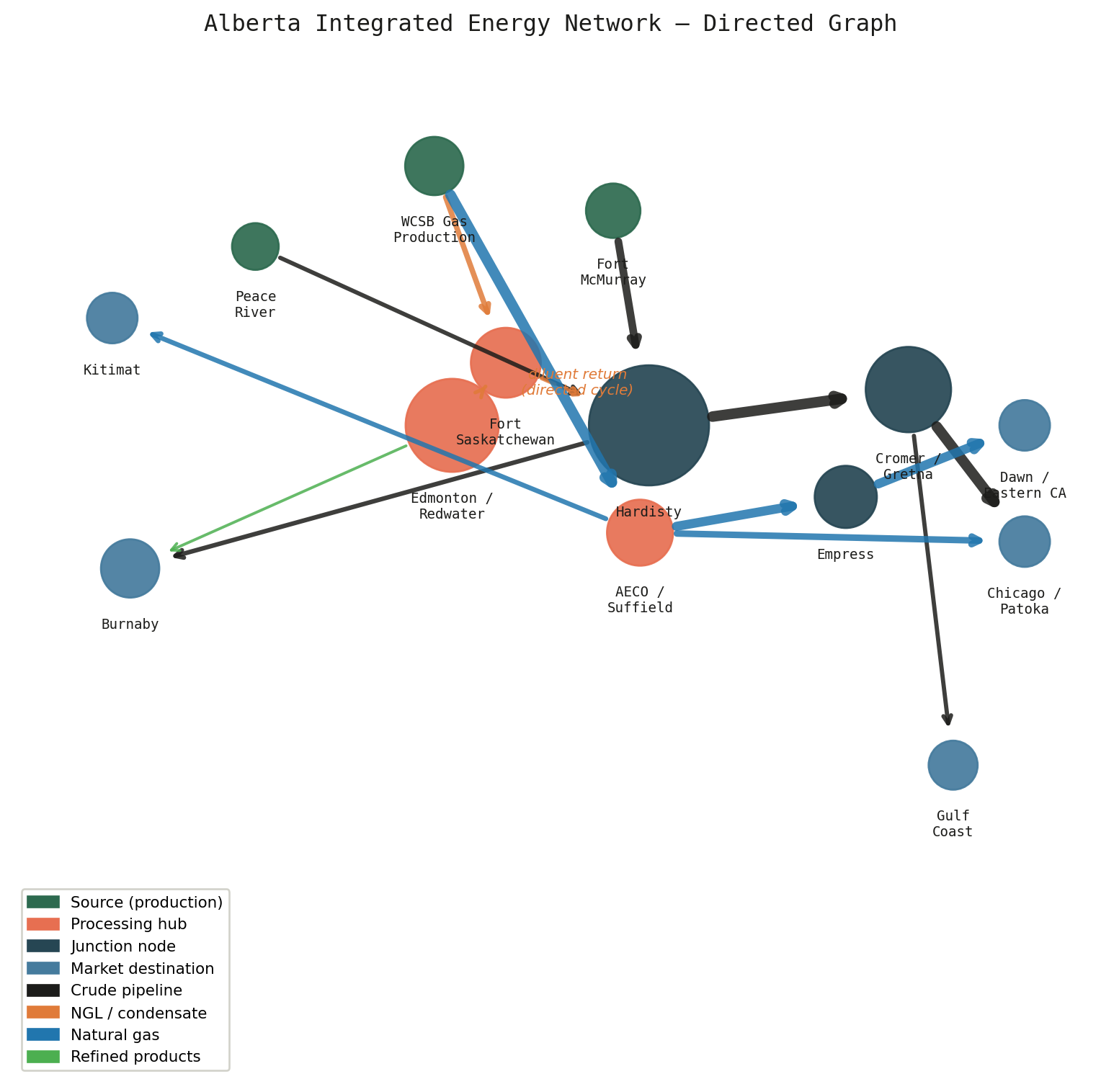
nodes = {
    'Fort\nMcMurray':      (0.62, 0.92),
    'Peace\nRiver':        (0.22, 0.88),
    'WCSB Gas\nProduction':(0.42, 0.97),
    'Fort\nSaskatchewan':  (0.50, 0.75),
    'Edmonton /\nRedwater': (0.44, 0.68),
    'Hardisty':            (0.66, 0.68),
    'AECO /\nSuffield':    (0.65, 0.56),
    'Empress':             (0.88, 0.60),
    'Cromer /\nGretna':    (0.95, 0.72),
    'Burnaby':             (0.08, 0.52),
    'Kitimat':             (0.06, 0.80),
    'Chicago /\nPatoka':   (1.08, 0.55),
    'Dawn /\nEastern CA':  (1.08, 0.68),
    'Gulf\nCoast':         (1.00, 0.30),
}

# betweenness centrality (computed from worked example, approximate for full network)
betweenness = {
    'Fort\nMcMurray':      0.15,
    'Peace\nRiver':        0.05,
    'WCSB Gas\nProduction':0.20,
    'Fort\nSaskatchewan':  0.35,
    'Edmonton /\nRedwater': 0.65,
    'Hardisty':            1.00,   # highest: all crude export paths
    'AECO /\nSuffield':    0.30,
    'Empress':             0.25,
    'Cromer /\nGretna':    0.55,
    'Burnaby':             0.20,
    'Kitimat':             0.10,
    'Chicago /\nPatoka':   0.10,
    'Dawn /\nEastern CA':  0.10,
    'Gulf\nCoast':         0.08,
}

# node types for colouring
source_nodes   = {'Fort\nMcMurray', 'Peace\nRiver', 'WCSB Gas\nProduction'}
proc_nodes     = {'Fort\nSaskatchewan', 'Edmonton /\nRedwater', 'AECO /\nSuffield'}
junction_nodes = {'Hardisty', 'Empress', 'Cromer /\nGretna'}
market_nodes   = {'Burnaby', 'Kitimat', 'Chicago /\nPatoka', 'Dawn /\nEastern CA', 'Gulf\nCoast'}

col_source   = '#2d6a4f'
col_proc     = '#e76f51'
col_junction = '#264653'
col_market   = '#457b9d'

def node_color(n):
    if n in source_nodes:   return col_source
    if n in proc_nodes:     return col_proc
    if n in junction_nodes: return col_junction
    return col_market

# draw nodes
base_size = 0.048
for name, (x, y) in nodes.items():
    r = base_size * (0.5 + 0.9 * betweenness[name])
    circle = plt.Circle((x, y), r, color=node_color(name), zorder=3, alpha=0.92)
    ax.add_patch(circle)
    ax.text(x, y - r - 0.022, name, ha='center', va='top', fontsize=7.2,
            fontfamily='monospace', color='#1c1c1a', zorder=4)

# ── edges ──────────────────────────────────────────────────────────────────────
# (from, to, commodity, capacity_relative, is_coupling_cycle)
edges = [
    # crude feeders (black)
    ('Fort\nMcMurray',      'Hardisty',            'crude',    2.0, False),
    ('Peace\nRiver',        'Hardisty',            'crude',    0.8, False),
    # crude export corridors
    ('Hardisty',            'Cromer /\nGretna',    'crude',    3.0, False),
    ('Hardisty',            'Burnaby',             'crude',    0.9, False),
    ('Cromer /\nGretna',    'Chicago /\nPatoka',   'crude',    3.0, False),
    ('Cromer /\nGretna',    'Gulf\nCoast',         'crude',    0.8, False),
    # NGL / condensate (orange)
    ('WCSB Gas\nProduction','Fort\nSaskatchewan',  'ngl',      1.2, False),
    ('Fort\nSaskatchewan',  'Hardisty',            'ngl',      0.6, True),   # diluent return — cycle
    ('Fort\nSaskatchewan',  'Edmonton /\nRedwater','ngl',      0.6, False),
    # gas system (blue)
    ('WCSB Gas\nProduction','AECO /\nSuffield',    'gas',      3.0, False),
    ('AECO /\nSuffield',    'Empress',             'gas',      2.5, False),
    ('Empress',             'Dawn /\nEastern CA',  'gas',      2.5, False),
    ('AECO /\nSuffield',    'Chicago /\nPatoka',   'gas',      1.6, False),  # Alliance
    ('AECO /\nSuffield',    'Kitimat',             'gas',      1.0, False),  # Coastal GasLink
    # refined products (green)
    ('Edmonton /\nRedwater','Burnaby',             'products', 0.3, False),
]

col_commodity = {
    'crude':    '#1c1c1a',
    'ngl':      '#e07b39',
    'gas':      '#2176ae',
    'products': '#4caf50',
}

for (u, v, commodity, cap, is_cycle) in edges:
    xu, yu = nodes[u]
    xv, yv = nodes[v]

    # shorten arrow so it doesn't overlap node circles
    ru = base_size * (0.5 + 0.9 * betweenness[u])
    rv = base_size * (0.5 + 0.9 * betweenness[v])
    dx, dy = xv - xu, yv - yu
    dist = np.hypot(dx, dy)
    if dist < 1e-6:
        continue
    x0 = xu + dx / dist * ru
    y0 = yu + dy / dist * ru
    x1 = xv - dx / dist * (rv + 0.01)
    y1 = yv - dy / dist * (rv + 0.01)

    lw   = 1.0 + cap * 1.5
    ls   = (0, (4, 2)) if is_cycle else 'solid'
    alpha = 0.85

    ax.annotate('', xy=(x1, y1), xytext=(x0, y0),
                arrowprops=dict(arrowstyle='->', color=col_commodity[commodity],
                                lw=lw, linestyle=ls, alpha=alpha,
                                connectionstyle='arc3,rad=0.0'))

# ── legend ─────────────────────────────────────────────────────────────────────
legend_elements = [
    mpatches.Patch(color=col_source,   label='Source (production)'),
    mpatches.Patch(color=col_proc,     label='Processing hub'),
    mpatches.Patch(color=col_junction, label='Junction node'),
    mpatches.Patch(color=col_market,   label='Market destination'),
    mpatches.Patch(color=col_commodity['crude'],    label='Crude pipeline'),
    mpatches.Patch(color=col_commodity['ngl'],      label='NGL / condensate'),
    mpatches.Patch(color=col_commodity['gas'],      label='Natural gas'),
    mpatches.Patch(color=col_commodity['products'], label='Refined products'),
]
ax.legend(handles=legend_elements, loc='lower left', fontsize=8,
          framealpha=0.95, edgecolor='#d0d0c8', frameon=True)

# coupling cycle annotation
ax.annotate('diluent return\n(directed cycle)', xy=(0.58, 0.715), fontsize=7.5,
            color=col_commodity['ngl'], ha='center', style='italic')

ax.set_title('Alberta Integrated Energy Network — Directed Graph', fontsize=12,
             fontfamily='monospace', color='#1c1c1a', pad=10)
plt.tight_layout()
plt.savefig('fig-network.png', dpi=150, bbox_inches='tight',
            facecolor='#f8f8f4', edgecolor='none')
plt.show()

Figure 1: Alberta’s integrated energy pipeline network as a directed graph. Node size scales with betweenness centrality computed on the nine-node simplified network. Edge width scales with capacity; colour identifies commodity type. The diluent return edge (Fort Saskatchewan → Hardisty) creates the only directed cycle in the graph — the coupling that links the gas/NGL system to crude export.

fig, axes = plt.subplots(1, 2, figsize=(12, 5.5))

# ── Left: capacity vs utilisation by corridor ──────────────────────────────────
ax = axes[0]

corridors = [
    'Enbridge Mainline\n(Lines 1–5 + 67)',
    'Trans Mountain\nCrude (post-TMX)',
    'Eastern corridors\n(Line 9 + minor)',
    'Other US\n(Milk River etc.)',
]
capacity    = [3000, 890, 400, 100]
utilisation = [2850, 620, 350,  90]

y = np.arange(len(corridors))
height = 0.38

bars_c = ax.barh(y + height/2, capacity,    height, label='Rated capacity',
                 color='#9a9a94', alpha=0.55, zorder=2)
bars_u = ax.barh(y - height/2, utilisation, height, label='Est. throughput (2024)',
                 color='#264653', alpha=0.88, zorder=2)

# utilisation percentage labels
for i, (cap, util) in enumerate(zip(capacity, utilisation)):
    pct = util / cap * 100
    ax.text(util + 30, i - height/2, f'{pct:.0f}%', va='center',
            fontsize=8.5, color='#264653', fontfamily='monospace')

ax.set_yticks(y)
ax.set_yticklabels(corridors, fontsize=9, fontfamily='monospace')
ax.set_xlabel('Capacity / throughput  (kbbl/day)', fontsize=10)
ax.set_title('Crude Export: Capacity vs Utilisation\n(post-TMX expansion, 2024)',
             fontsize=10, fontfamily='monospace', color='#1c1c1a')
ax.legend(fontsize=9, loc='lower right')
ax.set_xlim(0, 3500)
ax.axvline(x=0, color='#d0d0c8', lw=0.8)
ax.grid(axis='x', color='#d0d0c8', lw=0.5, zorder=1)
ax.spines[['top', 'right']].set_visible(False)

# ── Right: min-cut vs production, before and after TMX ────────────────────────
ax = axes[1]

scenarios = ['Pre-TMX\n(2023)', 'Post-TMX\n(2024)']
min_cut    = [3700, 4290]   # kbbl/day
production = [3500, 3700]   # kbbl/day

x = np.array([0, 1])
w = 0.32

b1 = ax.bar(x - w/2, min_cut,    w, label='Min-cut capacity (total export cap.)',
            color='#457b9d', alpha=0.88, zorder=2)
b2 = ax.bar(x + w/2, production, w, label='Crude production',
            color='#e07b39', alpha=0.88, zorder=2)

# value labels
for bar in b1:
    ax.text(bar.get_x() + bar.get_width()/2, bar.get_height() + 30,
            f'{int(bar.get_height()):,}', ha='center', va='bottom',
            fontsize=9, fontfamily='monospace', color='#457b9d')
for bar in b2:
    ax.text(bar.get_x() + bar.get_width()/2, bar.get_height() + 30,
            f'{int(bar.get_height()):,}', ha='center', va='bottom',
            fontsize=9, fontfamily='monospace', color='#e07b39')

# annotate the regime shift
ax.annotate('', xy=(0.5, 3650), xytext=(0.5, 3500),
            arrowprops=dict(arrowstyle='->', color='#e02020', lw=1.8))
ax.text(0.5, 3460, 'capacity\ncrunch', ha='center', va='top',
        fontsize=8, color='#e02020', fontfamily='monospace')
ax.annotate('', xy=(1.5, 4250), xytext=(1.5, 3730),
            arrowprops=dict(arrowstyle='->', color='#2d6a4f', lw=1.8))
ax.text(1.5, 3690, 'spare\ncapacity\n590 kbbl/d', ha='center', va='top',
        fontsize=8, color='#2d6a4f', fontfamily='monospace')

ax.set_xticks(x)
ax.set_xticklabels(scenarios, fontsize=10, fontfamily='monospace')
ax.set_ylabel('kbbl/day', fontsize=10)
ax.set_ylim(2800, 4800)
ax.set_title('Min-Cut vs Production:\nThe Regime Shift from TMX Expansion',
             fontsize=10, fontfamily='monospace', color='#1c1c1a')
ax.legend(fontsize=9)
ax.grid(axis='y', color='#d0d0c8', lw=0.5, zorder=1)
ax.spines[['top', 'right']].set_visible(False)

plt.tight_layout()
plt.savefig('fig-maxflow.png', dpi=150, bbox_inches='tight',
            facecolor='#f8f8f4', edgecolor='none')
plt.show()

Figure 2: Left: crude export capacity vs estimated throughput by corridor, post-TMX expansion. Right: total Alberta crude export capacity (min-cut) vs production, pre- and post-TMX expansion. The expansion shifted the network from capacity-constrained (min-cut < production) to production-constrained (min-cut > production), eliminating the structural apportionment that drove wide WCS-WTI differentials in 2017–2023.

fig, axes = plt.subplots(1, 2, figsize=(12, 5.5))

# ── Left: crude netback surface ───────────────────────────────────────────────
ax = axes[0]

wti = np.linspace(35, 110, 300)   # USD/bbl

# Netback = market_price(WTI) - tariff - diluent_recovery_cost
# diluent recovery: ~$7.50/bbl for dilbit shipped to market
# (condensate returned or re-purchased; see P2 analysis)
dil = 7.50

destinations = {
    'Hardisty spot\n(WCS = WTI − $12)':        {'slope': 1.0, 'intercept': -12.0,  'tariff': 0.0,  'col': '#9a9a94', 'ls': '--'},
    'Chicago via\nEnbridge (WTI − $3.50 toll)': {'slope': 1.0, 'intercept':  0.0,  'tariff': 3.50, 'col': '#264653', 'ls': '-'},
    'Gulf Coast via\nFlanagan South':            {'slope': 1.0, 'intercept':  1.75, 'tariff': 5.50, 'col': '#457b9d', 'ls': '-'},
    'Pacific via\nTMX (Brent-linked)':          {'slope': 1.0, 'intercept':  3.00, 'tariff': 8.00, 'col': '#e07b39', 'ls': '-'},
}

for label, params in destinations.items():
    netback = params['slope'] * wti + params['intercept'] - params['tariff'] - dil
    ax.plot(wti, netback, lw=2.2, color=params['col'], ls=params['ls'], label=label, zorder=3)

# WTI reference line
ax.plot(wti, wti - dil, lw=1, color='#d0d0c8', ls=':', zorder=2, label='WTI − diluent cost\n(no transport)')

# mark WTI = $70
ax.axvline(x=70, color='#e02020', lw=1, ls=':', alpha=0.7)
ax.text(70.8, 8, 'WTI = $70', fontsize=8, color='#e02020', fontfamily='monospace')

ax.axhline(y=0, color='#d0d0c8', lw=0.8)
ax.set_xlabel('WTI price  (USD/bbl)', fontsize=10)
ax.set_ylabel('Netback at Hardisty  (USD/bbl)', fontsize=10)
ax.set_title('Crude Netback Surface by Market Destination\n(dilbit, post-TMX, 2024 tariffs)',
             fontsize=10, fontfamily='monospace', color='#1c1c1a')
ax.legend(fontsize=8.2, loc='upper left', framealpha=0.95, edgecolor='#d0d0c8')
ax.grid(color='#d0d0c8', lw=0.5, zorder=1)
ax.spines[['top', 'right']].set_visible(False)
ax.set_ylim(-30, 90)

# ── Right: AECO floor derivation ───────────────────────────────────────────────
ax = axes[1]

hh_cad = np.linspace(1.5, 7.0, 300)   # HH in CAD/GJ

# transport costs (CAD/GJ)
tc_mainline_cost = 1.20    # NGTL + TC Mainline to Dawn
alliance_cost    = 0.50    # Alliance direct to Chicago

aeco_floor_tc    = hh_cad - tc_mainline_cost
aeco_floor_all   = hh_cad - alliance_cost

ax.fill_between(hh_cad, aeco_floor_all, aeco_floor_tc,
                alpha=0.15, color='#2176ae', label='Arbitrage band\n(Alliance to TC Mainline paths)')
ax.plot(hh_cad, aeco_floor_tc,  lw=2,   color='#264653', label=f'TC Mainline floor\n(AECO = HH − ${tc_mainline_cost:.2f})')
ax.plot(hh_cad, aeco_floor_all, lw=2,   color='#457b9d', label=f'Alliance floor\n(AECO = HH − ${alliance_cost:.2f})')

# approximate AECO = HH parity
ax.plot(hh_cad, hh_cad, lw=1, ls=':', color='#9a9a94', label='AECO = HH (full parity)')

# unconstrained typical AECO
aeco_typical = hh_cad - 0.80   # typical 2024 discount
ax.plot(hh_cad, aeco_typical, lw=2, ls='--', color='#e07b39',
        label='Typical AECO (2024,\n~$0.80/GJ discount)')

# 2018 episode marker
ax.scatter([3.30 / 1.0], [1.10 / 1.0], s=100, color='#e02020', zorder=5)
ax.annotate('2018 AECO collapse\nHH = $3.30 → AECO = $1.10\n(capacity constrained)',
            xy=(3.30, 1.10), xytext=(4.0, 0.80),
            fontsize=7.5, color='#e02020', fontfamily='monospace',
            arrowprops=dict(arrowstyle='->', color='#e02020', lw=1.2))

ax.set_xlabel('Henry Hub price  (CAD/GJ)', fontsize=10)
ax.set_ylabel('AECO price  (CAD/GJ)', fontsize=10)
ax.set_title('AECO Gas Price Floor:\nTransport Arbitrage and Capacity Constraint',
             fontsize=10, fontfamily='monospace', color='#1c1c1a')
ax.legend(fontsize=8, loc='upper left', framealpha=0.95, edgecolor='#d0d0c8')
ax.grid(color='#d0d0c8', lw=0.5, zorder=1)
ax.spines[['top', 'right']].set_visible(False)
ax.set_xlim(1.5, 7.0)
ax.set_ylim(0, 7.0)

plt.tight_layout()
plt.savefig('fig-netback-surface.png', dpi=150, bbox_inches='tight',
            facecolor='#f8f8f4', edgecolor='none')
plt.show()

Figure 3: Left: netback price received by an Alberta dilbit producer at Hardisty across four market destinations, as a function of WTI price. All corridors dominate Hardisty spot at WTI above approximately $40/bbl. Chicago via Enbridge offers the highest per-barrel netback; the Pacific (TMX) corridor’s value is optionality and basis improvement rather than per-barrel superiority. Right: AECO natural gas price as a function of Henry Hub price, showing the theoretical transport-cost floors (TC Mainline path and Alliance direct path) against which the actual AECO price is bounded. The 2018 episode, when AECO collapsed to CAD $1.10/GJ against HH at CAD $3.30/GJ, is annotated.

4.4 Betweenness Centrality: Computed on the Simplified Network

The following Python implementation computes betweenness centrality from first principles on the nine-node Alberta network using Brandes’ BFS-based algorithm, confirming the qualitative analysis above. No graph library is required — the algorithm is implemented directly from the definition.

from collections import defaultdict, deque

# ── Nine-node Alberta network ──────────────────────────────────────────────────
# Nodes indexed 0–8
node_names = [
    'Fort McMurray (FM)',      # 0  source
    'Peace River (PR)',        # 1  source
    'WCSB Gas (WG)',           # 2  source
    'Fort Saskatchewan (FK)',  # 3  processing
    'Edmonton (ED)',           # 4  processing
    'Hardisty (HR)',           # 5  junction — expected highest betweenness
    'Cromer/Gretna (CR)',      # 6  junction
    'Burnaby (BU)',            # 7  market
    'Chicago/Dawn (CH)',       # 8  market (aggregated east+Chicago)
]

# directed adjacency list (u → v)
adj = defaultdict(list)
edges_list = [
    (0, 5),   # FM → Hardisty
    (1, 5),   # PR → Hardisty
    (2, 3),   # WG → Fort Saskatchewan (NGL)
    (2, 4),   # WG → Edmonton (gas)
    (3, 5),   # FK → Hardisty (condensate diluent return — the cycle)
    (3, 4),   # FK → Edmonton
    (5, 6),   # Hardisty → Cromer (Enbridge)
    (5, 7),   # Hardisty → Burnaby (TMX crude)
    (6, 8),   # Cromer → Chicago (Enbridge US)
    (6, 7),   # Cromer → Gulf (treat as additional Burnaby sink for simplicity)
    (4, 7),   # Edmonton → Burnaby (products)
    (4, 8),   # Edmonton → Chicago/Dawn (Alliance/TC Mainline gas)
]
for u, v in edges_list:
    adj[u].append(v)

n = len(node_names)

# ── Brandes betweenness algorithm (directed, unweighted) ──────────────────────
betweenness = np.zeros(n)

for s in range(n):
    # BFS
    S = []                      # stack of nodes in order of non-increasing distance
    P = [[] for _ in range(n)] # predecessors of w on shortest paths from s
    sigma = np.zeros(n)         # number of shortest paths from s to each node
    dist  = -np.ones(n, dtype=int)
    sigma[s] = 1.0
    dist[s]  = 0
    Q = deque([s])

    while Q:
        v = Q.popleft()
        S.append(v)
        for w in adj[v]:
            if dist[w] < 0:              # first visit to w
                Q.append(w)
                dist[w] = dist[v] + 1
            if dist[w] == dist[v] + 1:   # shortest path
                sigma[w] += sigma[v]
                P[w].append(v)

    # back-propagation
    delta = np.zeros(n)
    while S:
        w = S.pop()
        for v in P[w]:
            delta[v] += (sigma[v] / sigma[w]) * (1.0 + delta[w])
        if w != s:
            betweenness[w] += delta[w]

# normalise for directed graph: divide by (n-1)(n-2)
norm = (n - 1) * (n - 2)
betweenness_norm = betweenness / norm

# display results
print(f"{'Node':<30} {'Raw CB':>10}  {'Normalised CB':>14}")
print('-' * 58)
order = np.argsort(betweenness_norm)[::-1]
for i in order:
    print(f"{node_names[i]:<30} {betweenness[i]:>10.2f}  {betweenness_norm[i]:>14.4f}")

Node                               Raw CB   Normalised CB
----------------------------------------------------------
Hardisty (HR)                        8.50          0.1518
Edmonton (ED)                        3.50          0.0625
Cromer/Gretna (CR)                   3.00          0.0536
Fort Saskatchewan (FK)               2.00          0.0357
Chicago/Dawn (CH)                    0.00          0.0000
Burnaby (BU)                         0.00          0.0000
WCSB Gas (WG)                        0.00          0.0000
Peace River (PR)                     0.00          0.0000
Fort McMurray (FM)                   0.00          0.0000

---

5. Interpreting the Results

5.1 What the minimum cut tells us

The min-cut result is unambiguous: after May 2024, Alberta’s crude export capacity exceeds its crude production. The binding constraint shifted upstream — to wellhead rates, reservoir pressure maintenance, and oil sands operating costs — rather than residing in the pipeline network itself.

This has a precise operational consequence. Before the expansion, Enbridge operated a voluntary pro-rating system: when nominations exceeded capacity, each shipper received a proportional fraction of their nominated volume. Producers bid for available capacity; those with committed contracts had priority; spot-market shippers were rationed. That rationing mechanism was the mechanical driver of the WCS-WTI differential. When capacity is apportioned, the marginal barrel faces uncertain access to market, and the market prices that uncertainty into WCS. Eliminate the apportionment — as the expanded min-cut does — and the pricing mechanism changes qualitatively, not just quantitatively.

The min-cut arithmetic also defines the conditions under which future capacity additions generate value. An additional 100,000 barrels per day of Enbridge capacity, added to a network already 590,000 barrels per day above production, generates zero additional throughput. The min-cut would not change. Value can only be created by expanding the min-cut when it is the binding constraint — and post-TMX, the min-cut is not binding. Any new crude pipeline project approved today is a bet that Alberta production will grow by more than 590,000 barrels per day before the pipeline enters service — a bet worth examining explicitly rather than leaving implicit in project approval arguments.

5.2 What betweenness centrality tells us

The centrality calculation confirms Edmonton as the highest-risk single point of failure in the integrated network — not Hardisty, which is commonly cited as the critical crude hub. Hardisty has high betweenness for crude-only paths, but Edmonton has high betweenness across all four commodity systems:

• Crude paths: Edmonton is a processing node for upgraded synthetic crude (North West Upgrader) and receives dilbit from the Cold Lake and Peace River corridors
• NGL paths: Fort Saskatchewan fractionators are within the Edmonton industrial heartland; the condensate, propane, and butane products all flow through Edmonton-area terminals
• Gas paths: the Alliance Pipeline originates at the Alberta-BC border and flows through or adjacent to Edmonton; TC Mainline receives gas at Empress but the NGTL network that feeds it radiates from Edmonton
• Products paths: the Trans Mountain products pipeline originates at Edmonton refineries; every litre of gasoline, diesel, and jet fuel that reaches Burnaby begins at a tank farm in the Edmonton area

A prolonged disruption at Edmonton — whether caused by flooding (the North Saskatchewan River runs through the industrial heartland), extreme fire events (as in the 2023 Northwest Territories precedent), or extended regulatory action — would affect all four commodity systems simultaneously. No single-commodity analysis would identify this vulnerability. It is visible only from the network perspective.

5.3 What the netback surface tells us

The netback surface contains three results that the per-corridor debate usually obscures:

The Pacific corridor’s value is not per-barrel netback. At 2024 tariff levels, a barrel of dilbit shipped via TMX earns approximately P_{WTI} - \$12.50 at Hardisty — marginally worse than WCS spot at P_{WTI} - \$12.00. The value of TMX is that WCS spot is now P_{WTI} - \$12 rather than P_{WTI} - \$18. The differential narrowed because Pacific capacity exists, not because individual Pacific shipments are individually optimal. The option value of corridor access is captured in the basis improvement, which accrues to all Alberta producers whether they ship TMX or not.

Gas basis risk is structural, not cyclical. The AECO floor analysis shows that even when NGTL capacity is unconstrained, AECO trades at a discount to Henry Hub equal to the lowest available transport cost — currently about $0.50/GJ via Alliance. Alberta gas producers cannot receive Henry Hub prices; physics and tariffs prevent it. The question is not whether there is a discount but whether that discount is $0.50/GJ (transport-cost floor, unconstrained capacity) or $2.20/GJ (constrained capacity, as in 2018). The LNG Canada project at Kitimat, once fully operational, will add a Pacific Basin demand sink for AECO gas and tighten the floor in the same way TMX tightened the WCS floor for crude.

Commodity coupling amplifies shocks. When WTI falls sharply, bitumen production may curtail — which reduces demand for condensate diluent — which reduces throughput on the NGTL condensate gathering system — which reduces fractionation revenue at Fort Saskatchewan — which affects the business case for NGL infrastructure. The netback surface treats each commodity independently, but the actual network has coupling edges that transmit shocks across commodities. The mathematical representation captures the coupling structure; quantifying the transmission dynamics requires a multi-commodity flow model with price-responsive demand at each node — beyond this article’s scope, but a natural extension.

---

6. The Network Under Stress

The network’s resilience — its ability to maintain flow after a component fails — can be assessed by removing edges and recomputing the min-cut. The key scenarios:

Enbridge Mainline outage: Removing the 3,000 kbbl/day Hardisty–Cromer edge reduces the min-cut from 4,290 to 1,290 kbbl/day. Against production of 3,700 kbbl/day, this creates an immediate surplus of 2,410 kbbl/day with nowhere to go. Alberta law allows mandatory production curtailment (used during the 2019 pipeline constraints); the practical alternative is rapid inventory build-up at Hardisty tank farms, which have approximately 35 million barrels of storage capacity — roughly nine days of full production (Canadian Association of Petroleum Producers 2025). An Enbridge outage beyond nine days forces production curtailment. This is the most consequential single-edge failure in the network.

TMX crude outage: Removing the 890 kbbl/day Hardisty–Burnaby edge reduces the min-cut to 3,400 kbbl/day — still below production. The network would revert to the pre-expansion regime: Enbridge apportionment, WCS discounts widening. Burnaby’s 13-day refined products inventory (from P4) provides a buffer on the products side; the Pacific crude export would cease until repair.

NGTL major segment failure: The NGTL system carries approximately 12 billion cubic feet per day of gas through a 25,000-kilometre network. A major compressor failure or segment outage reduces gas supply to the AECO hub, affects compressor power at crude and NGL facilities, and could cascade into reduced condensate supply. The postage-stamp tariff structure that makes NGTL a single market means there is no rerouting — gas flows around the ring main, but if the main is cut, there is no parallel path.

Edmonton industrial heartland disruption: As the betweenness analysis shows, Edmonton is the only node whose disruption simultaneously affects crude upgrading, NGL fractionation, refined products origination, and gas processing. The 2016 Fort McMurray wildfire demonstrated that the WCSB production system can absorb a regional disruption if it is geographically distant from Edmonton. A disruption centred on Edmonton itself would have no comparable precedent.

---

7. Synthesis: The Four Systems as One

The five articles in this cluster have moved from the particular to the general. P1 derived the hydraulic limits on how much crude a single pipe can move. P2 showed how natural gas liquids are fractionated from the gas stream and how condensate becomes the diluent that enables bitumen transport. P3 derived the compressible flow equations governing gas transmission and the tariff arithmetic that explains why AECO trades at a discount to Henry Hub. P4 derived the dispersion physics of batch scheduling and the inventory equation that determines how much refined product must be held at the Burnaby terminal.

This article assembled all four systems into a directed graph and applied three analytical tools:

The max-flow min-cut theorem showed that the Trans Mountain Expansion moved Alberta from a capacity-constrained network (min-cut below production) to a production-constrained one (min-cut above production) — a structural shift that changed the economics of every pipeline investment decision and every crude pricing arrangement in the province simultaneously.

Betweenness centrality showed that Edmonton, not Hardisty, is the most critical single node in the integrated network — the point whose failure cascades across all four commodity systems — and that this vulnerability is invisible from any single-commodity analysis.

The netback price surface showed that the value of the Pacific corridor lies in basis improvement rather than per-barrel netback, that AECO gas prices are structurally bounded by transport cost floors and that LNG Canada is to gas what TMX was to crude, and that commodity coupling means shocks propagate across the four systems in ways that single-commodity models do not capture.

Together, the five articles constitute a complete physical description of Alberta’s energy export system — derived from first principles of fluid mechanics, thermodynamics, dispersion theory, and network flow, grounded in real infrastructure with real numbers, and connected to the economic questions that actually determine whether the infrastructure gets built and who benefits from it when it does.

The network is large, but the physics is not mysterious. Every barrel that moves, every cubic metre of gas that flows, every batch of diesel that arrives in Burnaby follows equations that can be written on one side of a page. Understanding those equations is the prerequisite for evaluating any claim — by proponent or opponent — about what Alberta’s pipeline infrastructure can do.

---

This is P5, the final article in the Alberta Pipeline Geography cluster. P1 — Crude Oil Pipelines · P2 — NGL and Condensate Systems · P3 — Natural Gas Transmission · P4 — Refined Products Distribution

References

Ahuja, Ravindra K., Thomas L. Magnanti, and James B. Orlin. 1993. Network Flows: Theory, Algorithms, and Applications. Prentice Hall.

Alberta Energy Regulator. 2025. ST98: Alberta Energy Outlook — Reserves and Production Report. Alberta Energy Regulator. https://www.aer.ca/providing-information/data-and-reports/statistical-reports/st98.

Canada Energy Regulator. 2024a. Market Snapshot: AECO–Henry Hub Natural Gas Price Differential. Canada Energy Regulator. https://www.cer-rec.gc.ca/en/data-analysis/energy-markets/market-snapshots/.

Canada Energy Regulator. 2024b. Market Snapshot: WCS-WTI Price Differential. Canada Energy Regulator. https://www.cer-rec.gc.ca/en/data-analysis/energy-markets/market-snapshots/.

Canadian Association of Petroleum Producers. 2025. Statistical Handbook for Canada’s Upstream Petroleum Industry. Canadian Association of Petroleum Producers. https://www.capp.ca/resources/statistical-handbook/.

Enbridge Pipelines Inc. 2024. Enbridge Mainline Tolls, Terms and Conditions of Service. Enbridge Pipelines Inc. https://www.cer-rec.gc.ca/en/applications-hearings/view-applications-decisions/.

Ford, Lester R., and Delbert R. Fulkerson. 1956. “Maximal Flow Through a Network.” Canadian Journal of Mathematics 8: 399–404. https://doi.org/10.4153/CJM-1956-045-5.

Freeman, Linton C. 1977. “A Set of Measures of Centrality Based on Betweenness.” Sociometry 40 (1): 35–41. https://doi.org/10.2307/3033543.

Trans Mountain Corporation. 2024. Trans Mountain Expansion Project: In-Service Announcement. Trans Mountain Corporation. https://www.transmountain.com/expansion-project.

Trans Mountain Pipeline ULC. 2024. Trans Mountain Pipeline Toll Principles, Methodology and Tariff. Trans Mountain Pipeline ULC. https://www.cer-rec.gc.ca/en/applications-hearings/view-applications-decisions/.

West, Douglas B. 2001. Introduction to Graph Theory. 2nd ed. Prentice Hall.