The fractionation cascade, diluent supply chain, and the Cochin reversal
pipelines
NGL
fractionation
energy
Alberta
economic geography
Alberta’s oil sands produce bitumen that cannot flow through a pipeline without diluent. This article traces the million barrels per day of condensate that makes oil sands export possible — from gas plant extraction through the fractionation cascade to dilbit blending at Hardisty — and derives the mass balance mathematics governing separation through a Fort Saskatchewan fractionator.
You should know Basic chemistry: what hydrocarbons are, why some are gas at room temperature and some are liquid. What a boiling point is. Enough algebra to follow a balance equation.
You will learn How natural gas liquids are extracted from raw gas streams; how the fractionation cascade separates them into saleable products column by column; the vapor-liquid equilibrium mathematics that govern every separation; and how the pentanes-plus fraction — condensate — travels 700 kilometres from a gas plant near Grande Prairie to a dilbit blending station at Fort McMurray. You will also learn why a 2,900-kilometre pipeline built to carry propane eastward in 1978 was reversed in 2014 to carry condensate northward, and what that decision reveals about infrastructure and markets.
Why this matters P1 of this cluster derived the bitumen netback formula:
The P_{C5+} \cdot d term is not a minor rounding item. At a diluent ratio of d = 0.30 and condensate priced at USD 72/bbl, diluent cost consumes USD 21.60 per barrel of dilbit shipped — approximately 30–40% of the total delivered value under typical market conditions (Canada Energy Regulator 2024b). The present article explains what P_{C5+} represents physically, where the condensate comes from, and what controls its price and availability.
If this gets hard, focus on… The key insight is that hydrocarbons in a mixture boil at different temperatures, and a fractionation column exploits those differences to concentrate each component into a separate product stream. The mass balance equation is accounting: what enters must exit, distributed between an overhead distillate and a bottom product. The algebra that follows is arithmetic applied to that accounting constraint.
Forty kilometres northeast of Edmonton, where Highway 15 runs through flat farmland toward the Saskatchewan border, a cluster of silver and white columns rises from the prairie. The columns are distillation towers — some sixty metres tall, wrapped in insulation and instrumented with hundreds of sensors — and they are the industrial heart of what the Alberta Industrial Heartland Association calls Canada’s largest hydrocarbon processing region (Alberta Industrial Heartland Association 2024). Fort Saskatchewan and the surrounding communities host more than 40 major industrial facilities: ethylene plants, polypropylene units, styrene producers, and — at the base of the cascade that feeds them all — natural gas liquids fractionators.
Fractionators do one thing. They take a mixed stream of hydrocarbon liquids recovered from natural gas — ethane, propane, butanes, and condensate all jumbled together — and separate it into its components. Those components then flow into different destinies: ethane to crackers that turn it into ethylene and eventually plastic; propane into residential and commercial heating markets; butane to blending or petrochemical feedstock; condensate northward, eventually, as the diluent that makes oil sands bitumen shippable.
The connection between a fractionation column in Fort Saskatchewan and a barrel of diluted bitumen loading onto the Enbridge Mainline at Hardisty is indirect, invisible, and essential. Without the fractionation cascade, there is no diluent. Without diluent, the bitumen does not flow. The pipeline capacity that P1 derived from the Darcy-Weisbach equation is irrelevant if the product cannot meet specification at the injection point.
1. The Question
Three connected questions drive this article:
First: what are natural gas liquids, and how does a gas plant recover them from a raw wellhead gas stream?
Second: how does the fractionation cascade separate a mixed NGL stream into individual products — and what mathematics govern that separation at each column?
Third: how does condensate travel from a gas plant in the Montney or Deep Basin to an oil sands blending facility 700 kilometres away, and what happens when domestic supply falls short?
These are a chemistry question, a process engineering question, and a supply chain question. The answers are connected by the same physical fact: different hydrocarbon molecules have different boiling points, and pipeline infrastructure exists to exploit that difference in both directions — separating the mixture at the fractionator, then reassembling a specific blend at the dilbit injection point.
2. The Conceptual Model
Natural Gas Liquids: What They Are
Raw natural gas from a wellhead is not pure methane. It is a mixture of hydrocarbons ranging from methane (C_1, the lightest, a gas at all ambient conditions) through ethane (C_2), propane (C_3), butanes (C_4), and pentanes-plus (C_5^+, also called condensate). The heavier components are present in smaller proportions but have higher energy content and substantially higher market value per unit of energy (Canada Energy Regulator 2024b).
The normal boiling points set the sequence of everything that follows:
Component
Formula
Normal boiling point
State at 20°C, 1 atm
Methane
C_1H_4
−161°C
Gas
Ethane
C_2H_6
−89°C
Gas
Propane
C_3H_8
−42°C
Gas
Isobutane
i-C_4H_{10}
−12°C
Gas
Normal butane
n-C_4H_{10}
−1°C
Gas
Isopentane
i-C_5H_{12}
+28°C
Liquid
Normal pentane
n-C_5H_{12}
+36°C
Liquid
Hexane+ (C_6^+)
—
+69°C and above
Liquid
The pentanes-plus fraction — everything from C_5 upward — is liquid at ambient conditions and is called condensate in industry usage. It is this fraction that becomes diluent for oil sands bitumen.
The Recovery Step: From Raw Gas to Mixed NGL
At a gas processing plant, raw gas is first dehydrated and sweetened (water and hydrogen sulphide removed), then chilled to condense the heavier components. Two main recovery technologies are in use in Alberta:
Refrigeration and lean oil absorption — older technology, common in legacy plants. The gas is cooled to −30 to −40°C; C_3 and heavier components condense and are collected. Ethane recovery is partial. Widely used in the Foothills gas belt.
Cryogenic turboexpansion — the modern standard for high-recovery plants. The gas is chilled further, to −90°C or below, by expanding it through a turboexpander (a high-speed turbine that extracts energy as it drops the pressure). At these temperatures, C_2 and heavier components condense efficiently. Ethane recovery rates of 90–99% are achievable. Most new Montney and Deep Basin plants use this technology (Alberta Energy Regulator 2025).
The output of either process is a mixed NGL stream — sometimes called Y-grade or raw make — containing C_2 through C_5^+ in proportions that depend on the feed gas composition and the plant’s recovery targets. This mixed stream travels by pipeline to the fractionation hub. In Alberta, the primary destination is Fort Saskatchewan.
The Fractionation Cascade
A single distillation column cannot economically separate a four- or five-component mixture into pure products in one step. Instead, a cascade of columns is used, each removing one component from the top:
Deethanizer: overhead product is ethane (C_2); bottoms is C_3^+
Depropanizer: overhead is propane (C_3); bottoms is C_4^+
Debutanizer: overhead is mixed butanes (C_4); bottoms is condensate (C_5^+)
Butane splitter (optional): overhead is isobutane (i-C_4); bottoms is normal butane (n-C_4)
Each column exploits the boiling point difference between adjacent components. The condensate exiting the debutanizer bottoms is liquid at ambient temperature — no pressurisation required for storage or pipeline transport. It is then routed to oil sands producers as diluent feedstock.
3. Building the Mathematical Model
3.1 Vapor-Liquid Equilibrium and K-Values
A fractionation column works because, at any given temperature and pressure, a hydrocarbon mixture distributes its components unequally between the liquid and vapor phases. The equilibrium ratio, or K-value, describes this distribution:
K_i = \frac{y_i}{x_i}
where y_i is the mole fraction of component i in the vapor phase and x_i is its mole fraction in the liquid phase, both at equilibrium. A component with K_i > 1 prefers the vapor; K_i < 1 prefers the liquid.
For ideal mixtures — a reasonable first approximation for light hydrocarbon systems at moderate pressures — Raoult’s Law gives:
K_i = \frac{P_{\text{vap},i}(T)}{P}
where P_{\text{vap},i}(T) is the saturation vapor pressure of pure component i at temperature T, and P is the total system pressure. Components with higher vapor pressures (lower boiling points) have larger K-values and concentrate in the vapor phase.
Vapor pressures are calculated from the Antoine equation. In the form convenient for light hydrocarbons:
\log_{10} P_{\text{vap}} = A - \frac{B}{T + C}
where P_{\text{vap}} is in bar and T is in Kelvin. Published Antoine constants for ethane and propane are tabulated from the NIST WebBook; the Python implementation below uses these values directly.
Bubble point and dew point define the boundaries of the two-phase region at a given pressure:
Bubble point: the temperature at which the first bubble of vapor forms in a liquid of composition \{x_i\}. At bubble point: \sum_i K_i x_i = 1.
Dew point: the temperature at which the first drop of liquid condenses from a vapor of composition \{y_i\}. At dew point: \sum_i y_i / K_i = 1.
Between bubble point and dew point, vapor and liquid coexist. A fractionation column operates within this two-phase region at each theoretical stage.
3.2 Relative Volatility
The relative volatility\alpha_{ij} between two components i and j is the ratio of their K-values:
For ideal mixtures, \alpha_{ij} depends only on temperature (not pressure, since pressure cancels). Larger \alpha means a larger difference in volatility — easier separation, fewer stages required.
For a binary mixture with relative volatility \alpha = \alpha_{12} (component 1 more volatile), the VLE relationship simplifies to:
This is the equilibrium curve plotted on a McCabe-Thiele diagram. When \alpha = 1, the curve lies on the diagonal — no separation is possible. As \alpha increases, the curve bows further from the diagonal, and separation becomes progressively easier.
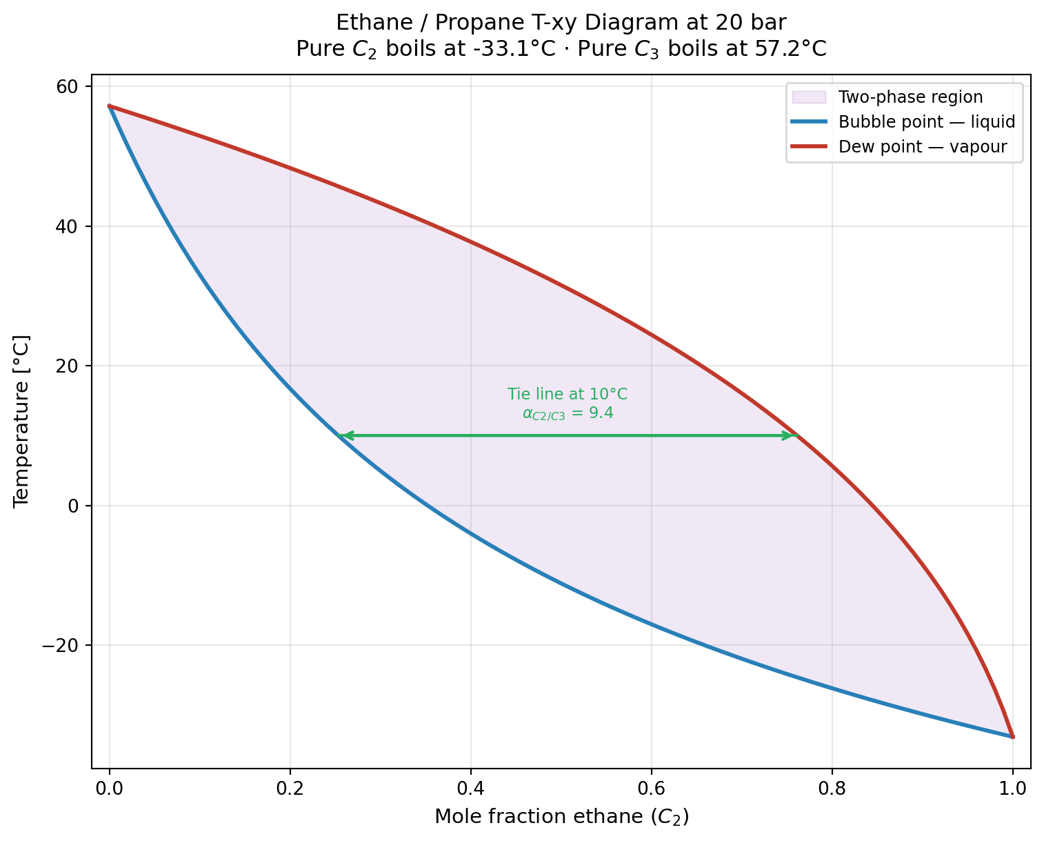
For the ethane/propane system at deethanizer conditions (20 bar, −30 to +50°C), \alpha_{C2/C3} ranges from approximately 5 at the warm reboiler end to 12 at the cold condenser end, with a column-average around 8. The figure below makes this geometric.
3.3 Overall and Component Mass Balance
For a distillation column operating at steady state, the overall mole balance across the column is:
F = D + B
where F is the feed molar flow rate, D is the distillate (overhead) flow, and B is the bottoms flow (all in kmol/day or any consistent unit).
For each component i, the component mole balance is:
F z_i = D x_{D,i} + B x_{B,i}
where z_i is the mole fraction of component i in the feed, x_{D,i} in the distillate, and x_{B,i} in the bottoms.
These two equations — overall and component — are the accounting framework for every column in the cascade. Given F, \{z_i\}, and the desired product specifications x_{D,i} and x_{B,i}, they determine D and B uniquely:
D = F \cdot \frac{z_i - x_{B,i}}{x_{D,i} - x_{B,i}}
The recovery of component i to the distillate — the fraction of the feed that ends up overhead — is:
The minimum number of theoretical separation stages at total reflux (the most favorable operating condition) is given by the Fenske equation(Fenske 1932):
LK = light key — the more volatile component targeted for the distillate (ethane in a deethanizer)
HK = heavy key — the less volatile component targeted for the bottoms (propane in a deethanizer)
x_{D,\text{LK}} = mole fraction of LK in distillate
x_{D,\text{HK}} = mole fraction of HK in distillate
x_{B,\text{LK}} = mole fraction of LK in bottoms
x_{B,\text{HK}} = mole fraction of HK in bottoms
\bar{\alpha}_{\text{LK/HK}} = geometric mean relative volatility between the column top and bottom
The Fenske equation is exact at total reflux for constant relative volatility. It gives the theoretical lower bound on column height. Actual columns require additional stages to achieve the same separation at finite reflux ratios — the Underwood equation(Underwood 1948) establishes the minimum reflux ratio, and the Gilliland correlation maps the relationship between actual reflux and actual stages. In practice, industrial deethanizers operate at reflux ratios of 2–4 times the minimum, with actual stage counts roughly twice N_{\min}.
3.5 Minimum Reflux: The Underwood Equation
The minimum reflux ratio R_{\min} — the lowest reflux at which the desired separation can theoretically be achieved with an infinite number of stages — comes from the Underwood equation (Underwood 1948):
where q is the feed quality (q = 1 for saturated liquid feed, q = 0 for saturated vapor), \alpha_i is the relative volatility of component i with respect to the heavy key, and \theta is found by solving for the root between the relative volatilities of the light and heavy keys. Then:
For a deethanizer with a liquid feed, q = 1, and the Underwood equation gives R_{\min} in the range of 0.5–2.0 depending on feed composition. Operating reflux R is typically set at (1.2–1.5) R_{\min} to balance energy cost against capital cost of column height.
3.6 The Diluent Blending Equation
The condensate produced from the debutanizer bottoms enters the diluent supply chain and eventually reaches an oil sands dilbit blending station. The blending arithmetic connects directly to P1’s netback model.
Let d be the diluent ratio — barrels of condensate per barrel of dilbit:
d = \frac{V_{\text{condensate}}}{V_{\text{dilbit}}} = \frac{V_{\text{condensate}}}{V_{\text{bitumen}} + V_{\text{condensate}}}
Alberta’s Enbridge Mainline specification requires dilbit density not exceeding 880–920 kg/m³ and viscosity not exceeding 350 centistokes at operating temperature (Enbridge Pipelines Inc. 2024). To meet these specifications, bitumen (density ~1,020 kg/m³, viscosity >10,000 cSt at 15°C) must be blended with condensate (density ~620–660 kg/m³, viscosity ~1–2 cSt). The resulting blend targets:
\rho_{\text{dilbit}} = \rho_{\text{bit}} (1-d) + \rho_{\text{C5+}} \cdot d
Solving for d given the target density of 890 kg/m³, bitumen at 1,020 kg/m³, and condensate at 640 kg/m³:
A diluent ratio of 0.30–0.35 is consistent with field practice and with the value used in P1 (Natural Resources Canada 2024). The slight variation reflects differences in bitumen grade (mining vs. SAGD), condensate composition, and seasonal temperature effects on viscosity.
At Alberta’s oil sands production rate of approximately 3.4 million barrels per day of bitumen, a diluent ratio of 0.30 implies:
But V_{\text{condensate}} = d \times V_{\text{dilbit}} = 0.30 \times (3{,}400{,}000 / 0.70) \approx 1{,}457{,}000 \times 0.30 \approx 437{,}000 bbl/day of condensate… Let me recalculate cleanly.
If we produce 3.4 million bbl/day of bitumen and the diluent ratio is d = 0.30 (30 bbl condensate per 100 bbl dilbit), then dilbit volume = 3{,}400{,}000 / (1 - 0.30) = 4{,}857{,}000 bbl/day, and condensate required = 4{,}857{,}000 \times 0.30 \approx 1{,}457{,}000 bbl/day (Canada Energy Regulator 2024b). Not all bitumen travels as dilbit — approximately 40% is upgraded to synthetic crude before export and requires no diluent — so the effective condensate demand is closer to 900,000–1,100,000 barrels per day of condensate for the dilbit portion.
4. Worked Example by Hand
Scenario: A Fort Saskatchewan deethanizer processes a mixed NGL feed of 10,000 kmol/day with the composition shown. Calculate the distillate and bottoms flows, the ethane recovery, and the minimum number of theoretical stages.
Feed composition:
Component
z_i
F z_i (kmol/day)
Ethane (C_2)
0.35
3,500
Propane (C_3)
0.35
3,500
Butane (C_4)
0.15
1,500
Pentanes+ (C_5^+)
0.15
1,500
Total
1.00
10,000
Specifications: distillate must contain 97 mol% ethane (x_{D,C2} = 0.97); bottoms must contain no more than 2 mol% ethane (x_{B,C2} = 0.02).
Relative volatility:\bar{\alpha}_{C2/C3} = 4.5 at average column conditions (geometric mean of condenser and reboiler values at 20 bar).
B = F - D = 10{,}000 - 3{,}474 = 6{,}526 \;\text{kmol/day}
Step 2 — Product composition check
Ethane in distillate: D \times x_{D,C2} = 3{,}474 \times 0.97 = 3{,}370 kmol/day Ethane in bottoms: F z_{C2} - D x_{D,C2} = 3{,}500 - 3{,}370 = 130 kmol/day Bottoms ethane mole fraction: 130 / 6{,}526 = 0.020 ✓ (meets specification)
Ethane recovery to distillate:3{,}370 / 3{,}500 = 96.3\%
Propane slips into distillate: (D - 3{,}370) / 3{,}500 = 0.030, so the distillate also contains 104 kmol/day propane. The bottoms is 3,396 kmol/day propane (97% of feed propane) plus all C_4 and C_5^+. This is correct behaviour — a deethanizer does not need to make a perfectly pure ethane distillate, only to separate ethane from the bulk of the heavier components for downstream processing.
Step 3 — Fenske minimum stages
For the deethanizer, the light key is C_2 and the heavy key is C_3:
A real deethanizer operating at 1.3 \times R_{\min} reflux would require approximately 2.5 \times N_{\min} \approx 11–12 theoretical stages, corresponding to 18–25 actual trays after accounting for a typical tray efficiency of 60–70%. This is consistent with the 20–28 tray deethanizers documented in the fractionation literature (Seader et al. 2011).
5. Computational Implementation
import numpy as npimport matplotlib.pyplot as pltfrom scipy.optimize import brentq# Antoine constants: log10(P_bar) = A - B / (T_K + C)# Source: NIST WebBook (ethane: 190–305 K; propane: 200–370 K)ANTOINE = {'C2': (4.51143, 791.300, 6.422),'C3': (4.53678, 1149.36, 24.906),}def P_vap(comp, T_K): A, B, C = ANTOINE[comp]return10.0** (A - B / (T_K + C)) # barP_sys =20.0# bar# Pure-component boiling points at P_sysT_C2 = brentq(lambda T: P_vap('C2', T) - P_sys, 150.0, 310.0) # KT_C3 = brentq(lambda T: P_vap('C3', T) - P_sys, 250.0, 400.0) # KN =100x1_arr = np.linspace(0.0, 1.0, N +1)y1_arr = np.linspace(0.0, 1.0, N +1)T_bub = np.zeros(N +1)y1_bub = np.zeros(N +1)T_dew = np.zeros(N +1)for i, x1 inenumerate(x1_arr): x2 =1.0- x1def bub_res(T):return x1 * P_vap('C2', T) + x2 * P_vap('C3', T) - P_sys T_b = brentq(bub_res, T_C2 -2, T_C3 +2) T_bub[i] = T_b y1_bub[i] = x1 * P_vap('C2', T_b) / P_sysfor i, y1 inenumerate(y1_arr): y2 =1.0- y1def dew_res(T): Pv2 = P_vap('C2', T) Pv3 = P_vap('C3', T)return y1 / Pv2 + y2 / Pv3 -1.0/ P_sys T_d = brentq(dew_res, T_C2 -2, T_C3 +2) T_dew[i] = T_d# T_bub is decreasing with x1; T_dew is decreasing with y1.# Build a common temperature grid for fill_betweenx.T_grid = np.linspace(T_C2, T_C3, 400)# At each T, find x1 on bubble curve and y1 on dew curvex_at_T = np.interp(T_grid, T_bub[::-1], x1_arr[::-1])y_at_T = np.interp(T_grid, T_dew[::-1], y1_arr[::-1])fig, ax = plt.subplots(figsize=(8, 6.5))ax.fill_betweenx(T_grid -273.15, x_at_T, y_at_T, alpha=0.12, color='#8e44ad', label='Two-phase region')ax.plot(x1_arr, T_bub -273.15, color='#2980b9', linewidth=2.2, label='Bubble point — liquid')ax.plot(y1_arr, T_dew -273.15, color='#c0392b', linewidth=2.2, label='Dew point — vapour')# Tie line example at T = 10°C (283 K)T_tie =283.15x_tie = np.interp(T_tie, T_bub[::-1], x1_arr[::-1])y_tie = np.interp(T_tie, T_dew[::-1], y1_arr[::-1])alpha_tie = (P_vap('C2', T_tie) / P_vap('C3', T_tie))ax.annotate('', xy=(y_tie, T_tie -273.15), xytext=(x_tie, T_tie -273.15), arrowprops=dict(arrowstyle='<->', color='#27ae60', lw=1.6))ax.plot([x_tie, y_tie], [T_tie -273.15, T_tie -273.15], color='#27ae60', linewidth=1.4, zorder=5)ax.text((x_tie + y_tie) /2, T_tie -273.15+1.8,f'Tie line at {T_tie -273.15:.0f}°C\n'r'$\alpha_{C2/C3}$'+f' = {alpha_tie:.1f}', ha='center', va='bottom', fontsize=8.5, color='#27ae60')ax.set_xlabel('Mole fraction ethane ($C_2$)', fontsize=11)ax.set_ylabel('Temperature [°C]', fontsize=11)ax.set_title('Ethane / Propane T-xy Diagram at 20 bar\n'f'Pure $C_2$ boils at {T_C2 -273.15:.1f}°C · Pure $C_3$ boils at {T_C3 -273.15:.1f}°C', fontsize=12, pad=10)ax.legend(fontsize=9, loc='upper right')ax.grid(alpha=0.3)ax.set_xlim(-0.02, 1.02)plt.tight_layout()plt.show()
Figure 1: T-xy diagram for the ethane/propane binary system at 20 bar — typical deethanizer operating pressure. The bubble point curve (blue) traces liquid compositions at phase boundary; the dew point curve (red) traces vapor compositions. The shaded two-phase region is where vapor and liquid coexist; within this region, the horizontal tie line connecting any liquid composition to its equilibrium vapor composition defines the separation achieved on one theoretical stage. The large temperature span (~90°C from pure ethane at −33°C to pure propane at +57°C) and the wide two-phase region reflect a relative volatility averaging ~8 across the column — a favourable separation.
import numpy as npimport matplotlib.pyplot as plt# FeedF =10_000.0# kmol/dayz = {'C2': 0.35, 'C3': 0.35, 'C4': 0.15, 'C5p': 0.15}FEED = {k: F * v for k, v in z.items()}# Recovery assumptions (fraction of component going overhead)# Deethanizerr_C2_DEE =0.963# C2 recovery to distillater_C3_DEE =0.030# C3 slip to distillate (small, unwanted)# Depropanizer (applied to DEE bottoms)r_C3_DEP =0.970# C3 recovery to distillater_C4_DEP =0.015# C4 slip to distillate# Debutanizer (applied to DEP bottoms)r_C4_DEB =0.980# C4 recovery to distillater_C5_DEB =0.010# C5+ slip to distillate# ── Deethanizer ──────────────────────────────────────────────────────────────DEE_dist = {'C2': FEED['C2'] * r_C2_DEE,'C3': FEED['C3'] * r_C3_DEE,'C4': 0.0,'C5p': 0.0,}DEE_bot = {k: FEED[k] - DEE_dist[k] for k in FEED}# ── Depropanizer ─────────────────────────────────────────────────────────────DEP_dist = {'C2': DEE_bot['C2'], # residual C2 goes overhead'C3': DEE_bot['C3'] * r_C3_DEP,'C4': DEE_bot['C4'] * r_C4_DEP,'C5p': 0.0,}DEP_bot = {k: DEE_bot[k] - DEP_dist[k] for k in FEED}# ── Debutanizer ──────────────────────────────────────────────────────────────DEB_dist = {'C2': 0.0,'C3': DEP_bot['C3'], # residual C3 overhead'C4': DEP_bot['C4'] * r_C4_DEB,'C5p': DEP_bot['C5p'] * r_C5_DEB,}DEB_bot = {k: DEP_bot[k] - DEB_dist[k] for k in FEED} # condensate!# ── Data for chart ────────────────────────────────────────────────────────────stages = ['Feed', 'Deethanizer\nbottoms', 'Depropanizer\nbottoms', 'Debutanizer\nbottoms\n(condensate)']flows = [FEED, DEE_bot, DEP_bot, DEB_bot]comps = ['C2', 'C3', 'C4', 'C5p']labels = ['Ethane ($C_2$)', 'Propane ($C_3$)', 'Butanes ($C_4$)', 'Pentanes+ ($C_5^+$) — condensate']colours = ['#3498db', '#e67e22', '#2ecc71', '#e74c3c']fig, axes = plt.subplots(1, 2, figsize=(13, 5.5), gridspec_kw={'width_ratios': [2.2, 1]})# Left: stacked horizontal bars for each stageax = axes[0]y_pos = np.arange(len(stages))bar_h =0.55lefts = np.zeros(len(stages))bar_handles = []for comp, label, colour inzip(comps, labels, colours): vals = np.array([f[comp] for f in flows]) b = ax.barh(y_pos, vals, bar_h, left=lefts, color=colour, label=label, alpha=0.88) bar_handles.append(b)# Annotate non-trivial barsfor i, (v, l) inenumerate(zip(vals, lefts)):if v >80: ax.text(l + v /2, i, f'{v:.0f}', ha='center', va='center', fontsize=7.5, color='white', fontweight='bold') lefts += valsax.set_yticks(y_pos)ax.set_yticklabels(stages, fontsize=10)ax.set_xlabel('Flow rate [kmol/day]', fontsize=10)ax.set_title('Mass Balance Through the Fractionation Cascade\n''Feed: 10,000 kmol/day mixed NGL', fontsize=11, pad=8)ax.legend(fontsize=8.5, loc='lower right')ax.grid(axis='x', alpha=0.3)ax.set_xlim(0, 11_000)ax.invert_yaxis()# Right: pie chart of condensate (debutanizer bottoms) compositionax2 = axes[1]cond_vals = [DEB_bot[c] for c in comps]cond_total =sum(cond_vals)cond_pct = [v / cond_total *100for v in cond_vals]# Only show slices with >0.5%plot_vals = [v for v in cond_vals if v / cond_total >0.002]plot_lbls = [f'{labels[i]}\n{cond_pct[i]:.1f}%'for i, v inenumerate(cond_vals) if v / cond_total >0.002]plot_clrs = [colours[i] for i, v inenumerate(cond_vals) if v / cond_total >0.002]wedges, _ = ax2.pie(plot_vals, colors=plot_clrs, startangle=90, wedgeprops={'alpha': 0.85})ax2.legend(wedges, plot_lbls, loc='lower center', bbox_to_anchor=(0.5, -0.28), fontsize=8)ax2.set_title(f'Condensate product\n({cond_total:.0f} kmol/day total)', fontsize=10)plt.tight_layout()plt.show()
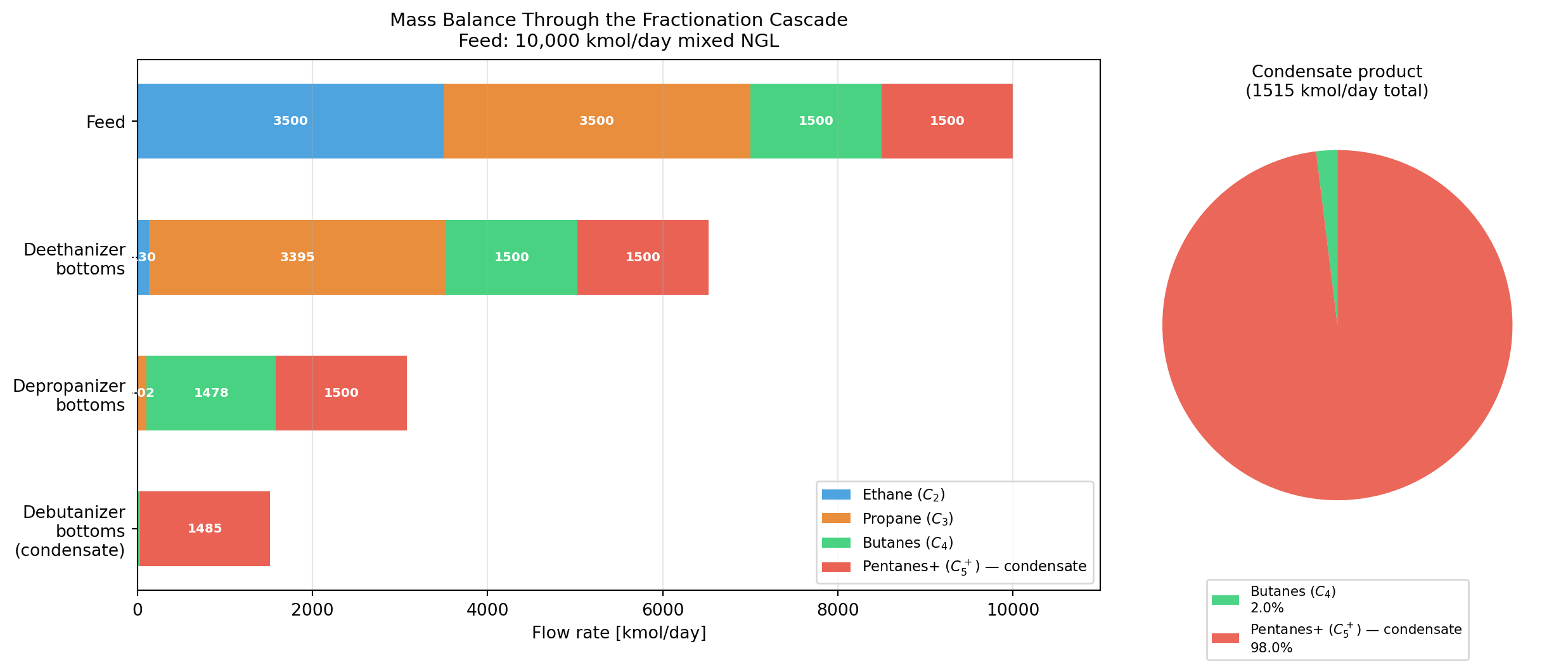
Figure 2: Mass balance through the three-column fractionation cascade for a representative Fort Saskatchewan NGL feed of 10,000 kmol/day. Each column removes one component overhead. After the deethanizer the ethane stream is routed to crackers or sales; after the depropanizer the propane stream enters heating and petrochemical markets; after the debutanizer, the butane stream goes to blending or export, and the pentanes-plus condensate at bottom — 1,500 kmol/day — becomes diluent feedstock for oil sands blending. The component-balance equations constrain every flow: what enters each column must exit in distillate plus bottoms. Small residual amounts of adjacent components in each stream reflect realistic 97–98% separation efficiency.
import numpy as npimport matplotlib.pyplot as plt# ── Netback model from P1 ─────────────────────────────────────────────────────d =0.30# diluent ratio# Enbridge corridor (Chicago, WCS-priced)WCS_enb =57.0# USD/bbl reference priceT_enb =7.00# USD/bbl total tariff# Trans Mountain corridor (Westridge, Brent-linked)WCS_tmu =63.0T_tmu =10.75# Netback as function of condensate priceP_C5_range = np.linspace(30, 100, 300)def netback(WCS, T, P_C5, d):return ((WCS - T) - P_C5 * d) / (1.0- d)NB_enb = netback(WCS_enb, T_enb, P_C5_range, d)NB_tmu = netback(WCS_tmu, T_tmu, P_C5_range, d)# Crossover where both netbacks are equalcross_idx = np.argmin(np.abs(NB_enb - NB_tmu))P_cross = P_C5_range[cross_idx]# Reference point from P1P_ref =72.0fig, (ax1, ax2) = plt.subplots(1, 2, figsize=(13, 5.5))# ── Left: netback sensitivity ─────────────────────────────────────────────────ax1.plot(P_C5_range, NB_enb, color='#2980b9', linewidth=2.2, label='Enbridge Mainline — Chicago (WCS)')ax1.plot(P_C5_range, NB_tmu, color='#e67e22', linewidth=2.2, label='Trans Mountain — Westridge (Brent-linked)')ax1.axvline(P_ref, color='#7f8c8d', linestyle='--', linewidth=1.2, label=f'P1 reference C5+ = USD {P_ref}/bbl')ax1.axvline(P_cross, color='#27ae60', linestyle=':', linewidth=1.5, label=f'Corridors equal at USD {P_cross:.0f}/bbl')ax1.axhline(0, color='#2c3e50', linewidth=0.8, linestyle='-')# Annotation of reference netbacksnb_enb_ref = netback(WCS_enb, T_enb, P_ref, d)nb_tmu_ref = netback(WCS_tmu, T_tmu, P_ref, d)ax1.plot(P_ref, nb_enb_ref, 'o', color='#2980b9', markersize=9, zorder=6)ax1.plot(P_ref, nb_tmu_ref, 's', color='#e67e22', markersize=9, zorder=6)ax1.annotate(f'USD {nb_enb_ref:.1f}/bbl', xy=(P_ref, nb_enb_ref), xytext=(P_ref -14, nb_enb_ref +2), arrowprops=dict(arrowstyle='->', color='#2980b9', lw=1.0), fontsize=8.5, color='#2980b9')ax1.annotate(f'USD {nb_tmu_ref:.1f}/bbl', xy=(P_ref, nb_tmu_ref), xytext=(P_ref +4, nb_tmu_ref +4), arrowprops=dict(arrowstyle='->', color='#e67e22', lw=1.0), fontsize=8.5, color='#e67e22')ax1.fill_between(P_C5_range, NB_enb, NB_tmu, where=(NB_tmu > NB_enb), alpha=0.10, color='#e67e22', label='TMX advantage region')ax1.fill_between(P_C5_range, NB_enb, NB_tmu, where=(NB_enb >= NB_tmu), alpha=0.10, color='#2980b9', label='Enbridge advantage region')ax1.set_xlabel('Condensate price $P_{C5+}$ [USD/bbl]', fontsize=10)ax1.set_ylabel('Bitumen netback [USD/bbl]', fontsize=10)ax1.set_title(f'Netback Sensitivity to Condensate Price\n'f'WCS={WCS_enb}, TMX ref={WCS_tmu}, diluent ratio d={d}', fontsize=11)ax1.legend(fontsize=7.8, loc='upper right')ax1.grid(alpha=0.3)ax1.set_ylim(-10, 65)# ── Right: diluent supply breakdown ───────────────────────────────────────────ax2.set_facecolor('#fafafa')# Notional supply numbers (approximate, based on CER NGL data)# Total diluent demand ~ 1,000,000 bbl/day# WCSB domestic condensate from gas plants: ~550,000 bbl/day# Synthetic crude substitution (upgrader output used as diluent): ~250,000 bbl/day# Cochin imports (condensate from US Bakken/Permian origin): ~95,000 bbl/day# Deficit bridged by imported condensate via truck/rail and other sources: ~105,000supply_labels = ['WCSB domestic\ncondensate\n(gas plant C5+)','Synthetic crude\nsubstitution','Cochin pipeline\nimports (US origin)','Other imports\n(rail, truck)',]supply_vals = [550, 250, 95, 105] # thousand bbl/daysupply_cols = ['#2980b9', '#27ae60', '#e74c3c', '#f39c12']bars = ax2.bar(range(len(supply_labels)), supply_vals, color=supply_cols, alpha=0.85, width=0.6, edgecolor='white')for bar, val inzip(bars, supply_vals): ax2.text(bar.get_x() + bar.get_width() /2, bar.get_height() +8,f'{val}k\nbbl/day', ha='center', va='bottom', fontsize=8.5, fontweight='bold')ax2.set_xticks(range(len(supply_labels)))ax2.set_xticklabels(supply_labels, fontsize=8.5)ax2.set_ylabel('Approximate supply volume [thousand bbl/day]', fontsize=10)ax2.set_title('Alberta Diluent Supply Stack\n''Notional breakdown — total demand ~1,000 kbbl/day', fontsize=11)ax2.set_ylim(0, 680)ax2.grid(axis='y', alpha=0.3)# Horizontal line at totalax2.axhline(sum(supply_vals), color='#2c3e50', linestyle='--', linewidth=1.2)ax2.text(len(supply_labels) -0.5, sum(supply_vals) +10,f'Total ≈ {sum(supply_vals)}k bbl/day', ha='right', fontsize=8.5, color='#2c3e50')plt.tight_layout()plt.show()
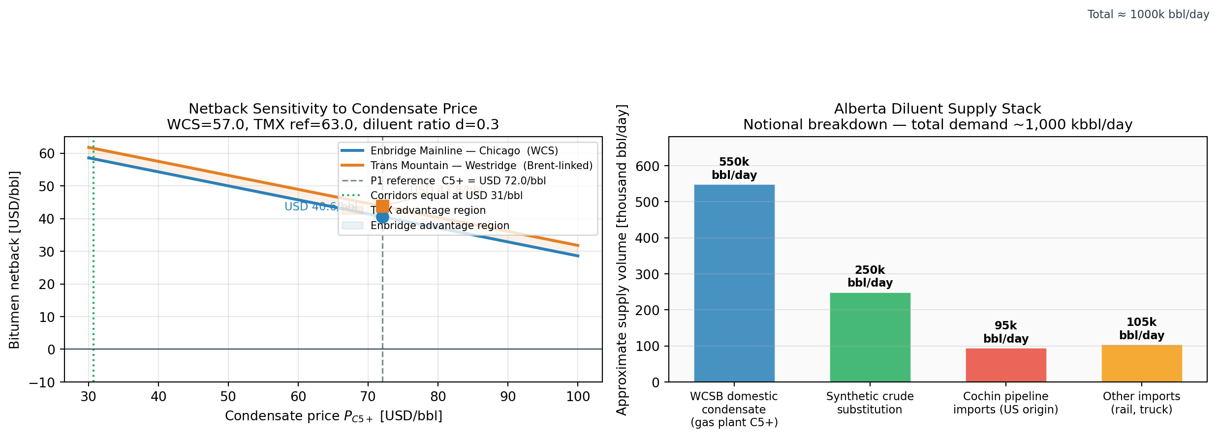
Figure 3: Left: Bitumen netback sensitivity to condensate (C5+) price, for the Enbridge and Trans Mountain corridors derived in P1. At the P1 reference point (C5+ = USD 72/bbl), the Trans Mountain corridor delivers USD 3.22/bbl more netback than Enbridge — but this advantage compresses rapidly if condensate prices rise, because Trans Mountain’s higher tariff leaves less headroom. The condensate price at which both corridors yield the same netback is marked. Right: notional Alberta diluent supply breakdown illustrating the structural dependence on Cochin imports and WCSB domestic production. Actual proportions vary year-to-year with Montney production, Cochin utilization, and upgrader synthetic crude substitution.
6. The Diluent Supply Chain
The mass balance above describes one fractionator. Alberta operates roughly 900 active gas processing plants, and more than 600 of them recover pentanes-plus fractions (Alberta Energy Regulator 2025). The aggregate condensate output of those plants — gathered by NGL liquids pipelines (sometimes called feeder lines or Y-grade lines), transported to fractionators at Fort Saskatchewan or other hubs, processed through the debutanizer cascade, and then re-routed by condensate pipeline toward Hardisty — constitutes the primary domestic diluent supply.
The journey involves several separate pipeline systems:
Y-grade gathering lines collect mixed NGL from gas plants across the WCSB and transport it to fractionation hubs. Pembina Pipeline’s networks in the Drayton Valley region, the Peace Pipeline system, and Alberta Energy Company’s gathering systems handle the bulk of this movement. Y-grade travels as a pressurised liquid — it contains enough light components (ethane, propane) to flash to vapor at ambient conditions and must be maintained above its bubble point throughout transport.
Condensate pipelines from fractionators to Hardisty carry the debutanizer bottoms product southward and eastward to the blending hub. The Enbridge system includes condensate-carrying segments within the Mainline right-of-way. Pembina and others operate dedicated condensate lines in the Fort Saskatchewan–Edmonton corridor.
The return diluent circuit — in principle but not universally in practice — sees condensate travel north with the dilbit batch, be separated at the destination refinery, and return to Alberta as recovered diluent. In reality, U.S. Midwest refineries typically prefer to retain the condensate fraction as refinery feedstock and sell it at local market prices. Alberta oil sands producers must therefore source fresh condensate continuously, not rely on a closed recycling loop (Canada Energy Regulator 2025).
This structural need — ongoing fresh condensate supply of 900,000 to 1,100,000 barrels per day, with no reliable return circuit — is what created the market conditions for the Cochin reversal.
7. The Cochin Reversal: Geography of a Reversed Decision
In 1978, a pipeline company built a 2,900-kilometre pipeline called Cochin, running from Fort Saskatchewan, Alberta, eastward through Saskatchewan and Manitoba to a terminal at Windsor, Ontario (National Energy Board 2015). Its purpose was to carry liquefied petroleum gas — primarily propane — from Alberta’s prolific gas plants to the Ontario market. Propane was a by-product of gas processing that had limited markets in the west and a ready market for heating and industrial use in the east. Cochin filled that arbitrage.
For three decades, it did. Then two things changed simultaneously.
First, Alberta gas processing technology improved. The shift from refrigeration to cryogenic turboexpansion, driven by high NGL value relative to methane, substantially increased propane and condensate extraction rates. Alberta’s propane supply grew faster than eastern demand could absorb.
Second, North American shale gas development — accelerating through the mid-2000s and sharply from 2010 onward — flooded the U.S. Midwest and Appalachian basins with associated NGLs from the Permian Basin, Bakken, Eagle Ford, and Marcellus formations. Propane markets in Ontario no longer needed western Canadian supply; local and U.S. sources were cheaper. Cochin’s eastbound business eroded.
But in the other direction, something was happening that Cochin’s original builders could not have anticipated. Oil sands production was growing toward two million, then three million barrels per day. Each barrel of dilbit required 30% condensate. Alberta’s domestic condensate production, while large, was not growing as fast as dilbit demand. The condensate price in Alberta began trading at a premium to condensate prices in U.S. Bakken and Williston Basin markets, where shale gas processing was generating enormous surpluses.
The arbitrage was clear. If condensate could be moved from Bakken origin points in North Dakota or Illinois through an existing pipeline to Hardisty, the price differential would cover the tariff and generate a profit. The pipeline already existed. It just needed to be reversed (Kinder Morgan Canada 2015).
Kinder Morgan Canada (the Cochin operator at the time) filed with the National Energy Board in 2012 and completed the reversal in mid-2014. The repurposed Cochin now carries light condensate northward from Aitkins Lake, Saskatchewan (connected to U.S. origin points via connecting pipelines) to Hardisty, Alberta — approximately 95,000 barrels per day. It is one of the more elegant examples in North American pipeline history of sunk infrastructure finding a second economic life when market conditions invert.
The Cochin reversal also illustrates the geographic structure of the diluent supply system. The condensate that travels north on Cochin originates partly in North Dakota’s Bakken formation and partly from Permian Basin condensate that has been fractionated, moved by NGL pipeline to Illinois, and then injected into the Cochin connection point. Alberta’s oil sands diluent supply is therefore partially dependent on U.S. shale gas processing economics — and on the price differential between Alberta condensate demand and Gulf Coast or Bakken supply, mediated by the Cochin tariff.
8. Interpretation
Why the fractionation hub concentrates where it does
Fort Saskatchewan’s position as the primary NGL fractionation hub reflects several geographic coincidences that have become structural advantages (Alberta Industrial Heartland Association 2024). The NOVA Gas Transmission system and its predecessor lines historically ran through or near the Edmonton area, making it a natural aggregation point for gas processing outputs. The proximity to oil sands markets (condensate goes north) and petrochemical demand (ethane goes to crackers, propane to markets) makes Fort Saskatchewan the lowest-cost hub for multiple commodity flows simultaneously. Once industrial infrastructure concentrates — pipelines, fractionators, crackers, storage — it generates agglomeration effects that reinforce concentration. The hub is where it is because it made sense decades ago, and it stays where it is because moving it would require reconstructing the network.
Condensate is a binding constraint, not a market footnote
The netback sensitivity chart above shows what happens when condensate prices rise. At USD 72/bbl, both corridors are commercially viable. At USD 95/bbl, the Trans Mountain corridor’s netback advantage over Enbridge narrows to near zero; at USD 100+/bbl, both corridors approach marginal viability depending on WCS pricing. A sustained condensate price spike does not primarily signal a problem with pipeline infrastructure — it signals a problem with the diluent supply chain upstream of the pipeline.
In practice, condensate prices in Alberta are highly correlated with crude oil prices but also exhibit their own tightness episodes. The 2022 condensate market tightening — driven by simultaneous Montney supply disruptions, elevated oil sands production targets, and compressed Cochin volumes during a maintenance period — briefly pushed Alberta condensate premiums above USD 10/bbl over WTI equivalents, materially impressing the netback for dilbit producers (Canada Energy Regulator 2024a).
Synthetic crude as partial diluent substitute
Upgrading bitumen to synthetic crude, as approximately 40% of oil sands output is processed, eliminates the diluent requirement entirely. SCO (32–34° API, 0.3–0.8% sulphur) flows without any additive and commands a quality premium over dilbit at destination refineries. The share of SCO versus dilbit in Alberta’s total export mix is therefore not purely a technical or refinery preference question — it is also influenced by condensate availability and price. When condensate is tight, the economic advantage of the upgrader route (no diluent cost) increases. When condensate is cheap, the dilbit route’s lower capital cost makes it more competitive. The two routes are partial substitutes in the diluent market, moderating but not eliminating condensate price swings.
9. What Could Go Wrong
WCSB condensate production decline
Alberta’s domestic condensate supply is tied to Montney and Deep Basin gas production, which also produces associated condensate from the well stream. The Montney has been growing, but growth rates are sensitive to gas prices, royalty regimes, and capital availability. A sustained low gas price environment that curtails Montney drilling would reduce not only gas supply but also the condensate that the gas processing plants recover. Because condensate is a by-product of gas production, not a primary target, the supply response to condensate price signals is slow — new wells must be drilled and completed, which takes 12–24 months.
LNG Canada and the condensate competition
LNG Canada’s Kitimat export facility, commissioning in 2024–2025, represents a new and large market for WCSB gas. Higher gas prices stimulated by LNG demand are generally positive for Montney drilling and therefore for condensate production. However, there is a competing effect: LNG plants and gas pipelines compete for lean, condensate-rich gas streams that processing plants need to extract NGL efficiently. At full LNG Canada utilisation of approximately 14 million tonnes per year (roughly 2.1 billion cubic feet per day of gas feed), the fraction of WCSB gas that passes through NGL-extracting plants rather than bypass lines may shift in ways that affect aggregate condensate extraction rates (Canada Energy Regulator 2024b).
Cochin tariff and capacity risk
The Cochin pipeline capacity of approximately 95,000 bbl/day is modest relative to total diluent demand (roughly 10% of the supply stack). But it is concentrated — Cochin is the primary source of non-domestic condensate, and a prolonged outage (mechanical failure, regulatory issue, or commercial dispute) would force diluent buyers to source from alternatives: rail imports, increased trucking, or curtailing dilbit production in favour of more synthetic crude. The 2020 Cochin tariff dispute between Kinder Morgan and the Canada Energy Regulator illustrates the regulatory risk embedded in a single-source supply component.
Temperature and viscosity: the winter diluent ratio problem
The diluent ratio d = 0.30 is a specification condition — it meets pipeline density and viscosity requirements at the temperature at which the line operates. In Alberta winters, soil temperatures at shallow pipeline depths can fall to −5 to −15°C along parts of the Mainline, increasing dilbit viscosity. To compensate, producers either increase the diluent ratio (consuming more condensate per barrel of bitumen) or heat the product before injection (consuming energy). Both responses have costs, and the condensate consumption increase tightens the diluent market exactly when cold weather is most likely to have disrupted gas plant operations that supply domestic condensate. The systems are coupled in the wrong direction from a supply-demand stability perspective.
10. Extension: The Petrochemical Downstream
The fractionation cascade produces not only condensate for oil sands diluent but also ethane, propane, and butane streams that anchor Alberta’s petrochemical industry. The Fort Saskatchewan complex is the feedstock origin for approximately CAD 16 billion worth of downstream chemical production (Alberta Industrial Heartland Association 2024).
Ethane from the deethanizer overhead travels by the Alberta Ethane Gathering System (AEGS) — a dedicated ethane pipeline network — to crackers operated by NOVA Chemicals (now INEOS) and Dow Chemical. Ethane crackers break the C_2H_6 molecule into ethylene (C_2H_4) and hydrogen under high-temperature steam cracking (>800°C). Ethylene is the world’s most widely produced organic chemical by volume and the feedstock for polyethylene, the most common plastic. Pembina’s Heartland Petrochemical Complex, completing construction through 2025, adds a propane dehydrogenation unit that converts propane to propylene — the feedstock for polypropylene (Pembina Pipeline Corporation 2024).
The feedstock cost structure matters to the economics of these plants. When condensate prices rise (as in a diluent tightness episode), the price of propane and ethane may also rise — they are produced in the same columns from the same feed stream, and the relative price of each component in the NGL barrel responds to aggregate demand pressure. Ethane crackers in Alberta are therefore exposed to the same supply dynamics as dilbit producers, even though their product — polyethylene pellets — bears no obvious connection to oil sands bitumen.
The integration of these downstream markets within the same geographic hub is not coincidental. Fort Saskatchewan exists where it does because co-locating the fractionation cascade, the crackers, and the condensate redistribution infrastructure reduces the per-unit cost of every product. The NGL cluster is a geographic fact before it is an industrial policy — the molecules leave the Montney wells bound for the same point by the physics of where gas pipelines economically aggregate.
11. Math Refresher: Why Equilibrium Stages Work
The concept of an ideal stage
A theoretical equilibrium stage (or theoretical plate) is a device in which vapor and liquid streams enter, mix to thermodynamic equilibrium, and exit as separate streams. On each such stage, the vapor leaving is in equilibrium with the liquid leaving — the K-values apply exactly.
Real column trays achieve roughly 60–75% of this theoretical separation (the tray efficiency). A column requiring 12 theoretical stages would use 18–20 actual trays to achieve the same separation. Packed columns are rated in height equivalent to a theoretical plate (HETP) — typically 0.3–0.6 metres for hydrocarbon service — and a 12-stage column would be 4–7 metres of packing.
Why the Fenske exponent is a logarithm
Starting from a single stage with relative volatility \alpha, the enrichment ratio in the distillate versus the bottoms for the light key is approximately \alpha per stage. Over N stages at total reflux, the enrichment accumulates multiplicatively:
N \approx \frac{\ln\!\left(\dfrac{x_{D,\text{LK}}}{x_{D,\text{HK}}} \cdot \dfrac{x_{B,\text{HK}}}{x_{B,\text{LK}}}\right)}{\ln \alpha}
This is the Fenske equation. The logarithm appears because separation accumulates by multiplication across stages — the same reason compound interest is calculated with exponentials. Each theoretical plate multiplies the separation ratio by \alpha; taking the log converts that multiplication into the addition that gives the linear stage count.
The practical consequence: doubling the separation difficulty (squaring the separation factor) requires only a 2× increase in the number of stages, not a 4× increase — because stages contribute additively in log-space. This is what makes fractionation an economically efficient separation technology: the capital cost scales roughly linearly with stage count, but the separation difficulty scales as the logarithm.
Connecting back to the pipeline system
The fractionation cascade is not merely a processing step between a gas plant and a pipeline. It is the mechanism by which a single raw material stream — mixed NGL from hundreds of individual gas wells — is disaggregated into components that serve entirely different markets: a plastic feedstock (ethane), a heating fuel (propane), a gasoline blendstock (butanes), and a pipeline diluent (condensate). Each component exits the cascade and enters a separate infrastructure that optimises its delivery to a different demand centre.
The mass balance equations that govern each column are simple. Their economic consequence — determining what fraction of Alberta’s gas production generates diluent value versus chemical feedstock value versus fuel value — is what makes the fractionation hub the most economically complex site in Alberta’s energy infrastructure, even though its towers are considerably less visible in the public debate than the pipelines they supply.
\rho_{\text{dilbit}} = \rho_{\text{bit}}(1-d) + \rho_{C5+} d
Condensate fraction required
Netback (from P1)
(P_{\text{WCS}} - T - P_{C5+} d) / (1-d)
Effect of diluent cost on producer economics
The physical result that matters most: The fractionation cascade separates mixed NGL by exploiting boiling point differences stage by stage. The minimum number of stages required scales as the logarithm of the separation difficulty — each column is shorter than intuition suggests. At Fort Saskatchewan, three columns in sequence convert a heterogeneous mixture into four separate commodity streams, one of which is the condensate that makes oil sands export possible.
The economic result that matters most: Condensate is not a commodity footnote in the dilbit netback formula — it consumes approximately 30% of the delivered value of each barrel shipped. Its price is set by a global NGL market that neither Alberta producers nor the Canada Energy Regulator controls, and its supply is structurally connected to both Montney gas economics and U.S. shale condensate production via the Cochin pipeline. A disruption in any of these upstream systems propagates directly into the netback arithmetic derived in P1.
Next: P3 — Natural Gas Transmission — the NOVA Gas Transmission system, the Weymouth equation for compressible flow, and the AECO–Henry Hub basis differential derived from transport cost arithmetic.
Alberta Industrial Heartland Association. 2024. Alberta Industrial Heartland: Canada’s Petrochemical Centre. Alberta Industrial Heartland Association. https://www.albertaindustrialheartland.com/.